NuOscProbExact 1.11.0: exact neutrino oscillation probabilities for two, three, and now four flavors — on PyPI!

Standard

Documentation: https://mbustama.github.io/NuOscProbExact/

Notebooks: https://github.com/mbustama/NuOscProbExact/tree/main/notebooks

Source code: https://github.com/mbustama/NuOscProbExact

PyPI: https://pypi.org/project/nuoscprobexact/

Neutrino oscillation probabilities look like a solved problem until the Hamiltonian stops being the textbook one. There is a closed form in vacuum, and another in two-flavor constant-density matter, and after that it runs out. Add a realistic density profile, a non-standard interaction, a Lorentz-violating operator or a fourth state, and the usual options are to expand in a parameter that may not be small, to diagonalise the Hamiltonian numerically at every point of a grid, or to integrate the Schrödinger equation and hope the step was short enough.

NuOscProbExact does none of these. The Hamiltonian and the time-evolution operator are expanded in the basis of SU(2), SU(3) or SU(4) matrices, and exponentiated analytically using the closure of the algebra. What comes out is a closed form for the probabilities in terms of two or three invariants of the Hamiltonian: no eigenvectors, no numerical diagonalisation, no integration, and no approximation beyond floating-point round-off. Any Hermitian 2×2, 3×3 or 4×4 matrix will do, whatever physics put it there. The method is Ohlsson and Snellman’s, revisited in the 2019 paper; the extension to SU(4) is new since then.

Four flavors is where it stops, for a reason external to neutrino physics: at five, the eigenvalues stop being expressible in radicals — Abel–Ruffini — and the closed form ends with them. Four is exactly what 3+1 needs.

If your reference point is a numerical evolution code, the output is the same object — probabilities, or the evolution operator itself — but with no step size to converge and no dependency beyond numpy. I wrote the first version because adding a model should mean writing down a matrix, not writing a solver. Seven years on it does rather more than it did, and version 1.11.0 now installs with pip.

What it makes easy

  • Any model, without a new code path. Vacuum, matter, non-standard interactions, Lorentz-invariance violation, sterile states: none of these is a special case in the code. Each is a different matrix handed to the same routine.
  • A whole scan in one call. A curve against energy or baseline, or a full oscillogram over both, with no Python loop.
  • Neutrinos through the Earth. Along a zenith angle, or between two of fifteen named sites — CERN–Gran Sasso, Fermilab–Homestake, Tokai–Kamioka and others — with the density profile taken from PREM. Or through any hand-built sequence of slabs of arbitrary width and density, each solved exactly and the operators multiplied.
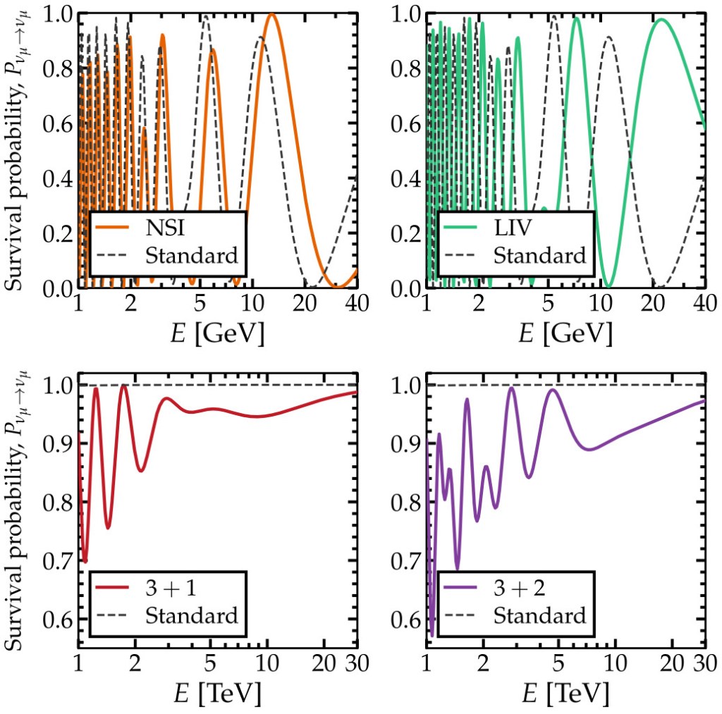
  • 3+1 sterile scenarios at four flavors, as closed four-state systems rather than as leakage out of the three-flavor block.
  • The evolution operator itself, not only probabilities, for composing across segments or propagating a density matrix.

Install with:

pip install nuoscprobexact

and, for the optional compiled backend:

pip install "nuoscprobexact[fast]"

MIT licence. Python 3.9 or newer, tested on 3.9 through 3.13, and numpy is the only required dependency: no compiler, nothing to build.

Main features

Accuracy

  • Cross-checked against independently written code. The probabilities agree with nuSQuIDS to round-off once conventions are matched, and the matter spectrum agrees with the Zaglauer–Schwarzer closed form.
  • A regression suite of 596 tests, at 100% coverage.

Speed

  • Arrays instead of loops. Stacks of Hamiltonians, arrays of baselines, or both broadcast together: roughly 20x to 90x faster than the equivalent Python loop, with no extra dependency.
  • An optional compiled backend. With numba installed, the batched paths run as compiled kernels — answers identical to round-off, used only where it has been measured to win.

What you need to provide

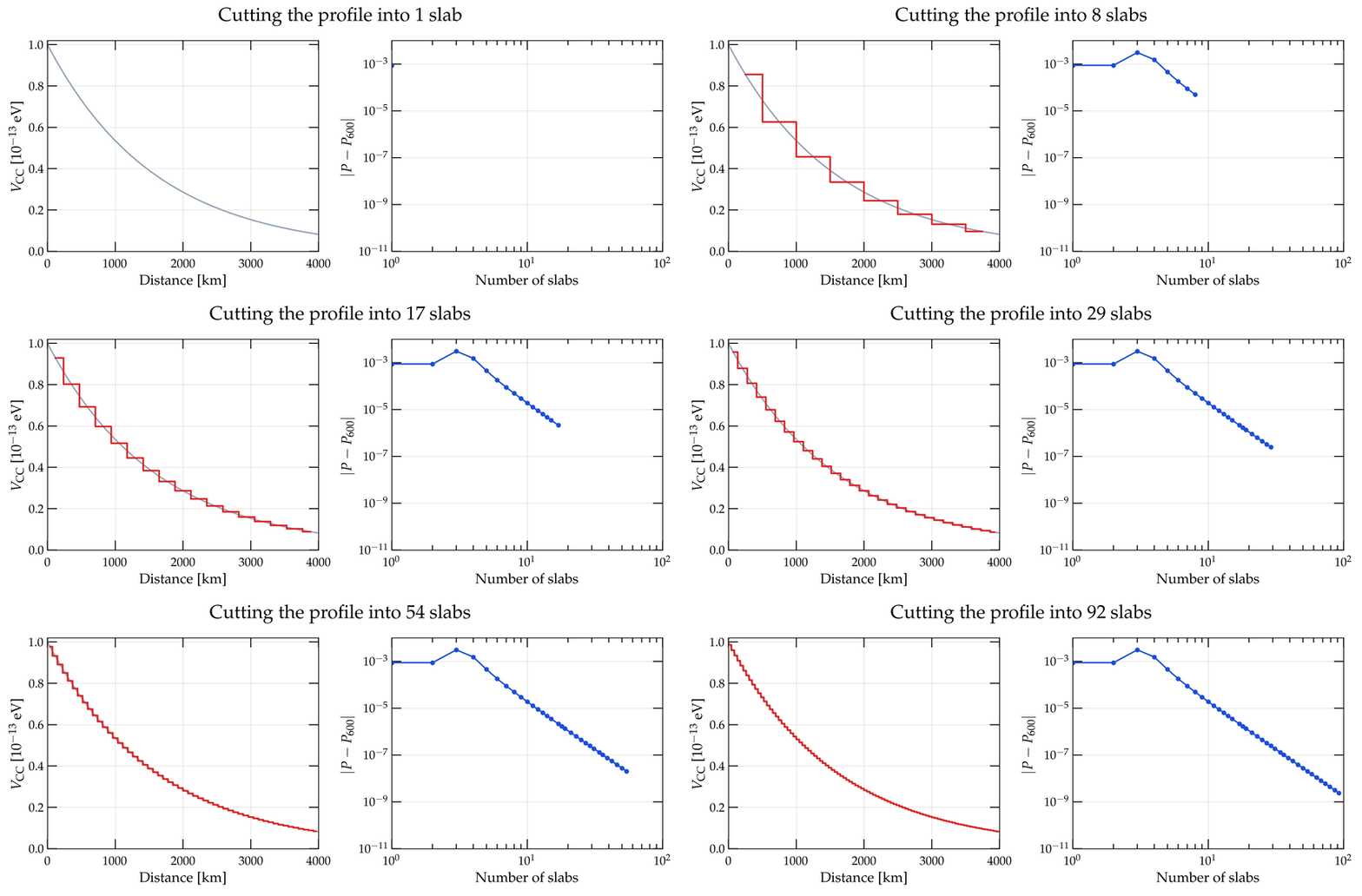
You provide a Hermitian matrix and a baseline, built by hand or with one of the bundled builders for the standard cases. The package returns the exact evolution operator and the probabilities that follow from it, and stops there: no fluxes, no cross sections, no detector response, no fitting. One assumption is worth stating plainly: the Hamiltonian is taken to be time-independent over each segment. A smoothly varying profile can be slabbed, but the step size is then set by the oscillation rather than by the density, and there the documentation points at a Magnus-type method instead.

A minimal example

import numpy as np
import oscprob3nu
import hamiltonians3nu
from globaldefs import *
# The vacuum Hamiltonian, without the 1/E factor, so an energy scan
# computes it once
h_vac = hamiltonians3nu.hamiltonian_3nu_vacuum_energy_independent(
S12_NO_BF, S23_NO_BF, S13_NO_BF, DCP_NO_BF, D21_NO_BF, D31_NO_BF)
# One probability, at 1 GeV over 1300 km
Pee, Pem, Pet, Pme, Pmm, Pmt, Pte, Ptm, Ptt = oscprob3nu.probabilities_3nu(
np.asarray(h_vac)/1.e9, 1300.0*CONV_KM_TO_INV_EV)
print('Pee = %.5f, Pem = %.5f, Pet = %.5f' % (Pee, Pem, Pet))

prints

Pee = 0.92768, Pem = 0.01432, Pet = 0.05800


(The quickstart goes through this more slowly; the recipes page has short, complete snippets for most of what the package can compute, each with real output.)

What is new since 1.0.0

The original announcement, in May 2019, covered the method paper and the code on GitHub. The method has not changed since; almost everything around it has. Whole-array scans arrived in 1.2.0, the optional numba backend in 1.6.0, the Earth and arbitrary layered matter in 1.8.0, and four flavors — oscprob4nuhamiltonians4nu, the SU(4) expansion — in 1.9.0. In 1.11.0, a non-Hermitian Hamiltonian raises instead of quietly returning probabilities that still sum to one. Along the way, a documentation site and eighteen worked notebooks.

One thing to flag for anyone still running 1.0.0: two fixes in 1.1.0 changed numbers, both at two flavors. probabilities_2nu was missing the h2 contribution to P(νe → νμ), which is invisible whenever the off-diagonal entry is real — so vacuum and constant-density matter were unaffected, but a CP-violating two-flavor Hamiltonian was not — and the two-flavor vacuum Hamiltonian used the opposite sign convention, invisible in vacuum and consequential once a matter potential is added. Three-flavor results from 1.0.0 are unaffected; the changelog has the details.

Some physics it’s meant for

Long-baseline accelerator experiments. DUNE-like baselines through the crust, with matter effects and the CP phase, and the bi-probability ellipses above, which show how matter pushes neutrinos and antineutrinos off the CP-symmetric diagonal. Notebook 05.

Atmospheric neutrinos through the Earth. Zenith-angle scans with the density taken from PREM rather than from a single average value, which is where the mass ordering and the θ23 octant separate. Notebooks 07 and 12.

Sterile neutrinos, 3+1. Short-baseline appearance and disappearance, and the sterile matter resonance through the Earth, with the four states treated as a closed, unitary system rather than as leakage out of the three-flavor block. Notebook 16.

Non-standard interactions and Lorentz-invariance violation. Both enter as extra Hermitian terms added to the vacuum Hamiltonian, so a new operator means a new matrix, not a new solver. Notebook 03.

Unusual matter profiles. Castle-wall and other hand-built profiles, where the arrangement of the matter changes the answer even when the mean density does not — a parametric-resonance effect no constant-density approximation can show. Notebook 08.

PyFC: a Python framework for Feldman-Cousins confidence intervals

Standard

Links

Setting a confidence interval sounds like a solved problem, until you actually have to do it. Deciding whether to quote a two-sided interval or a one-sided upper limit after looking at the data — the classic “flip-flopping” — breaks coverage, and near a physical boundary (a mass, a cross section, a flavor fraction) the usual construction can return an empty or unphysical interval. Feldman and Cousins’ 1998 unified approach fixed this by using the likelihood-ratio ordering principle to let the data decide the interval’s shape automatically, with guaranteed coverage throughout. It has become the standard approach for small-signal counting experiments across particle and astroparticle physics — but implementing it correctly, especially in more than one dimension and with realistic, finite-statistics systematics, is a substantial piece of software to get right.

That’s what I built PyFC to handle — it supports binned and unbinned likelihoods natively, in the same framework, rather than treating one as a special case of the other. Given a likelihood, it runs the Monte Carlo pseudo-experiments needed to empirically calibrate the profile-likelihood-ratio distribution, and returns exact-coverage Feldman-Cousins intervals and contours — in one or several dimensions, on a laptop or on a cluster. I kept needing exactly this — correct-coverage contours for neutrino mixing-parameter extractions and HNL coupling limits in my own papers — and rewriting the toy-generation machinery from scratch for each project wasn’t sustainable.

If your reference point is ROOT/RooStats’ FeldmanCousins calculator: PyFC does the same statistical job with no ROOT dependency — plain NumPy/SciPy arrays and a pip install, so it drops straight into a normal Python analysis.

Main features

PyFC is built for speed, flexibility, and accuracy — none traded off for the others.

Speed

  • Parallel processing by default. Binned fits use Numba/NumPy C-extensions with GIL-bypassing thread pooling; unbinned fits parallelize across CPU cores via Python’s multiprocessing (ProcessPoolExecutor). Toy generation — normally the bottleneck in any Feldman-Cousins analysis — scales with however many cores you give it.
  • No wasted compute. Adaptive early-stopping (adaptive_toys) and batched dispatch (toy_batch_size) stop generating toys once the result is statistically clear, instead of running a fixed, oversized number every time.
  • Resumable. Checkpointing saves state after each parameter/pair scan, so a run killed by a cluster walltime limit picks up where it left off instead of restarting from zero.

Flexibility

  • Native binned and unbinned support, in one framework. Poisson binned data — including arbitrary N-dimensional, even non-contiguous, histograms — and Extended Unbinned Maximum Likelihood models are both first-class, not one bolted onto the other.
  • A choice of optimizer. Gradient-based SciPy (L-BFGS-B), nested sampling via UltraNest, brute-force grid scans, or a Hybrid strategy that uses UltraNest’s robustness for the one global fit and SciPy’s speed for the many conditional fits that follow.
  • Physical constraints between parameters, not just per-parameter boxes. bounds_func and constraints express joint or simplex conditions (e.g. a + b ≤ 1) that an independent [lo, hi] range per parameter can’t capture.

Accuracy

  • Coverage that’s actually exact. The test-statistic distribution is derived empirically from generated toys rather than assumed from Wilks’ theorem, and disconnected accepted regions are reported as separate intervals instead of being silently merged into one.
  • Finite-Monte-Carlo corrections for limited simulation statistics, so a small MC background template doesn’t bias the result.

Also: optional 2D grid sparsification for faster contours, and an interactive CLI for generating run configurations.

Open source (GPLv3), Python 3.8+.

What you need to provide

You bring the physics, PyFC handles the statistics:

  • A physics mapper — for binned data, a compute_rates_func that maps your free parameters to expected bin counts and variances; for unbinned data, that plus pdf_components (one function per signal/background component) and a generate_toy_func for parametric bootstrapping.
  • Your data — a histogram (any shape, any dimension) or an array of events.
  • grids — the scan grid for each free parameter, plus bounds_func/constraints for any joint constraints between them.
  • A config — confidence level, toy settings, checkpointing, and the optimizer strategy (gridscipyultranest, or hybrid), built interactively with the CLI or as a JSON file.

Call compute_fc_intervals and PyFC takes care of the rest: toy generation, parallelization, checkpointing, and exact-coverage intervals out the other end — no hand-rolled Monte Carlo loop required.

A minimal example

For a binned Poisson analysis with a signal and a background component:

import numpy as np
from numba import njit
from pyfc import compute_fc_intervals
# A fixed expected-shape array, captured via closure (not itself a fit parameter)
expected_shape = np.array([0.1, 0.5, 2.0, 5.0])
@njit(fastmath=True, nogil=True)
def compute_rates(params):
"""Map parameters -> expected bin counts (mu) and variances (sigma2)."""
mu = params[0] * params[1] * expected_shape + params[2] # signal (rate x efficiency) + background
sigma2 = mu # Poisson variance
return mu, sigma2
observed_counts = np.array([20, 7, 2, 0]) # data — any shape, not just 1D
grids = [
np.linspace(1e-9, 1e-7, 20), # param_1
np.linspace(2.0, 3.0, 15), # param_2
np.linspace(0.8, 1.2, 10), # param_3
]
# results: exact-coverage FC intervals/contours for param_1-3, plus the
# underlying profile-likelihood scan and toy statistics behind them
results = compute_fc_intervals(
data=observed_counts,
grids=grids,
compute_rates_func=compute_rates,
**config, # confidence level, toy settings, strategy — see Configuration
)

(See the Quick Start Guide for the full binned and unbinned walkthroughs, with real output.)

Install with:

pip install PyFeldmanCousins

Some physics it’s meant for

Feldman-Cousins intervals matter most exactly where physics tends to live: near a boundary, with a marginal signal, where Gaussian/Wilks assumptions don’t hold. A few non-trivial cases PyFC is a natural fit for:

  • Astrophysical neutrino flavor composition. The flavor fractions (f_e, f_μ, f_τ) of the diffuse high-energy neutrino flux live on a simplex, f_e + f_μ + f_τ = 1 — precisely the joint-constraint case that bounds_func/constraints were built for. Feldman-Cousins contours on the flavor triangle are the standard way to compare an IceCube-like measurement against competing production scenarios (pion decay, muon-damped decay, neutron decay) and BSM flavor physics. Worked through hands-on in tutorial notebook 06.
  • Heavy Neutral Lepton searches at beam-dump experiments. A null result from a fixed-target experiment like SHiP constrains the active-sterile mixing |U|² as a function of HNL mass — an upper limit sitting right against the |U|² ≥ 0 boundary, often with disconnected sensitivity islands where the excluded region reappears at higher mass — see tutorial notebook 04 for how PyFC reports these correctly.
  • Dark matter direct-detection cross-section limits. The textbook case: a handful of candidate events over an uncertain background, where the interval needs to turn two-sided smoothly if a real excess ever shows up, instead of flip-flopping into an artificially tight one. The quickstart tutorial notebook works through essentially this case end to end.
  • Accelerator and reactor neutrino oscillations. Joint 2D regions on (Δm², sin²2θ) — this is literally the original 1998 Feldman-Cousins worked example, and still a good stress test for comparing the grid, SciPy, and Hybrid strategies — see tutorial notebook 05.
  • Neutrinoless double-beta decay. Binned searches for a peak near the Q-value, where the finite-MC correction matters because the simulated background templates are themselves statistics-limited — see tutorial notebook 04 for the correction on vs. off.

Measuring neutrino mixing above 1 TeV with astrophysical neutrinos

Standard

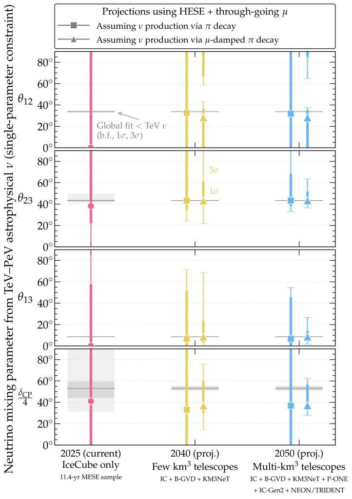
Today, the values of the neutrino mixing angles that govern flavor transitions are known to percent precision (the Dirac CP-violation phase is known much more poorly). However, these values are inferred exclusively from sub-TeV neutrino experiments. No measurement of the mixing parameters exists at the TeV scale and above. There, new-physics effects whose intensity grows with neutrino energy could modify the effective neutrino mixing. High-energy astrophysical neutrinos, with TeV-PeV energies, are primed for such measurements.

In a new paper with Qinrui Liu and Gabriela Barenboim, we have assessed in detail the power in these neutrinos to test mixing above 1 TeV, today and in the future. Concretely, we have extracted values of the four neutrino mixing angles (𝛉12, 𝛉23, 𝛉13) and the CP-violation phase (δCP) from the flavor composition of high-energy astrophysical neutrinos, i.e., the proportion of electron, muon, and tau neutrinos in their diffuse flux.

We extract present bounds on the mixing parameters from the 11.4-year IceCube Medium Energy Starting Events (MESE) sample, published in 2025. We find that the uncertainty in the measurement is too large to claim meaningful sensitivity to the mixing parameter.

For our projections, we use multi-neutrino-telescope combinations using projected detection rates at existing (IceCube, Baikal-GVD, KM3NeT) and future (P-ONE, IceCube-Gen2, NEON, TRIDENT, HUNT) neutrino telescopes. For these, we combine High Energy Starting Events (HESE) and through-going muons. Our projections show clear sensitivity to 𝛉23 and 𝛉13 (and, if neutrino production occurs via muon-damped pion decay, to δCP). This establishes benchmarks for the minimum size that new-physics modifications to the mixing parameters must have in order to be detectable.

Read more at:

Measuring neutrino mixing above 1 TeV with astrophysical neutrinos
Mauricio Bustamante, Qinrui Liu, Gabriela Barenboim
2602.14308 hep-ph

Testing Lorentz invariance with a flare of high-energy astrophysical neutrinos

Standard

Lorentz invariance is one of the pillars of modern physics, underlying special relativity—and, with that, the Standard Model—and general relativity. It posits that the laws of physics are the same for all observers moving in their own inertial frame. Yet, at high energies and short distances, Lorentz invariance may no longer hold.

To date, Lorentz invariance remains unbroken in all experimental tests. If it were violated, however, it could have many and varied consequences. Accordingly, there have been multiple searches for Lorentz invariance violation, using atom interferometry, gamma rays, cosmic rays, and neutrinos, etc. See, for instance, the data tables in 0801.0287.

High-energy astrophysical neutrinos, with TeV-PeV, are powerful probes of Lorentz invariance, thanks to their high energies and long traveled distances from their sources to Earth, of Mpc-Gpc scales. If Lorentz invariance is violated, it could imply that, en route to Earth, higher-energy neutrinos would travel more slowly than lower-energy neutrinos.

In a new paper, we introduce methods to look for these temporal distortions. We use the high-energy joint time and energy distribution of the neutrino flare detected by IceCube in 2014/2015 from the blazar TXS 0506+056 to look for specific signatures from Lorentz-invariance violation. We do this by borrowing non-parametric statistical methods previously used to look for signs of Lorentz-invariance violation in the gamma rays from gamma-ray bursts (1807.00189).

And, in doing so, we account for the significant energy and directional uncertainty associated to the detection of high-energy astrophysical neutrinos. Doing this makes our analysis realistic and robust, even if it erodes some of its sensitivity.

As a result, we set new lower limits on the energy scale of Lorentz-invariance violation in neutrino propagation. If Lorentz invariance is broken, this must happen at energies beyond 10^{14} GeV, if the effects depend linearly on the neutrino energy, or beyond 10^9 GeV, if they depend quadratically on it.

Read more at:

Probing Lorentz invariance with a high-energy neutrino flare
Mauricio Bustamante, John Ellis, Rostislav Konoplich, and Alexander S. Sakharov
2408.15949 astro-ph

Discovering Majorons from the neutrinos of the next galactic supernova

Standard

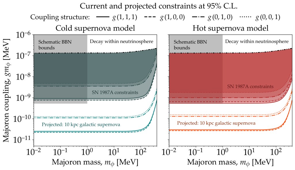
In the hot, dense cores of core-collapse supernova, neutrinos could coalesce to make new, heavy particles, like Majoron-like bosons, with masses from tens of MeV to more than 100 MeV. After escaping the supernova, these Majorons would decay into energies comparable to the parent Majoron mass, far more energetic than the standard supernova neutrinos emitted from the neutrinosphere, and arriving at Earth later than them.

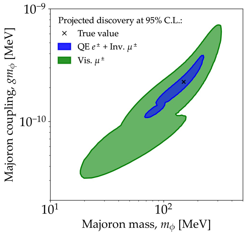
Thanks to large upcoming neutrino detectors, we might observe these high-energy neutrinos from the next galactic core-collapse supernova. Combining all available detection channels provides us with information on the energy, flavor, and arrival times of these neutrinos.

In a new paper, led by NBI PhD student Bernanda Telalovic, we have shown for the first time that we can combine this information use to clearly distinguish neutrinos from Majoron decay from the standard neutrinos of the next galactic supernova.

And, on top of that, we fold in the large uncertainty that exists in supernova physics by using two sophisticated supernova simulations (hot and cold) from the Garching group, obtained for two different assumptions for the mass of the proto-neutron star. However, our results do not hinge on us knowing what the real model, since we marginalize over it.

Should we detect no high-energy neutrinos, we will be able to place upper bounds on the Majoron coupling to neutrinos that are more than an order of magnitude stronger than the ones inferred from the observation of neutrinos from SN 1987A:

We show explicitly how the bounds are different depending on the flavor texture of the Majoron.

Conversely, should we detect high-energy neutrinos with late arrival times (tens of seconds post-bounce), we will be able to measure the mass and flavor-universal coupling of the Majoron:

Read more at:

The next galactic supernova can uncover mass and couplings of particles decaying to neutrinos
Bernanda Telalovic, Damiano F.G. Fiorillo, Pablo Martíinez-Miravé, Edoardo Vitagliano, Mauricio Bustamante
2406.15506 astro-ph

New limits on neutrino decay from high-energy astrophysical neutrinos

Standard

In the Standard Model, neutrinos are effectively stable, their lifetimes orders of magnitude longer than the age of the Universe. In proposed extensions of the Standard Model, however, neutrinos might decay faster, and so observing them decay would constitute evidence of new neutrino physics.

Regardless, neutrino lifetimes, even augmented by new physics, are likely very long, and the effects of decay are likely manifest only in neutrinos that travel a long distance, during which the chances of them decaying becomes appreciable even if they are long-lived.

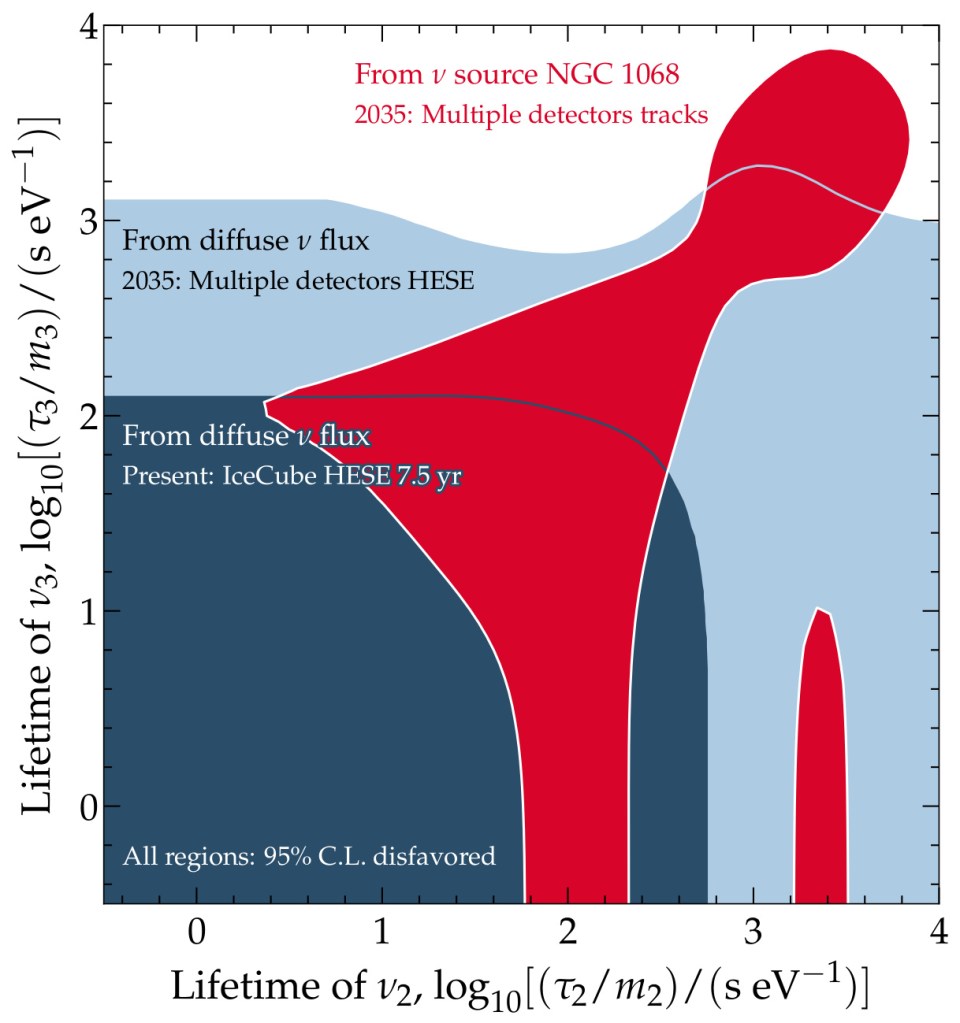
In a new paper, we have searched for signs of neutrino decay using the neutrinos from farthest away: the high-energy astrophysical neutrinos detected by IceCube, which travel cosmological-scale distances of Mpc-Gpc from their sources to Earth. Neutrino decay, in principle, alters the shape of the neutrino energy spectrum—introducing a step-like jump—and the flavor composition of the neutrinos upon reaching Earth—taking it outside the region expected from standard oscillations alone.

We find no signs of decay in present-day IceCube data, but place new, competitive lower limits on the lifetimes of the nu_2 and nu_3 neutrino mass eigenstates. We report, for the first time, limits inferred using the neutrinos from the first candidate steady-state astrophysical source of high-energy neutrinos, the active galaxy NGC 1068, and limits inferred from the diffuse flux of high-energy neutrinos.

These are arguably the most robust neutrino lifetime bounds garnered from high-energy astrophysical neutrinos so far! In addition, we make forecasts for the year 2035, combining multiple upcoming neutrino telescopes.

While similar studies have been performed before, ours brings two new perspectives, often overlooked or understudied, that make our results robust.

First, we consider broadly the large astrophysical uncertainties that plague the prediction of the flux of high-energy astrophysical neutrinos. This includes the size and shape of the neutrino energy spectrum, the flavor composition of the neutrino flux, the number or source populations and their distribution in redshift, and whether we have prior constraints on the size of the neutrino flux normalization. The impact of considering these uncertainties ranges from appreciable to critical. In some cases, they nearly make the sensitivity to neutrino decay vanish! Surprisingly, with present data, it is not possible to constrain neutrino decay using neutrinos from NGC 1068 due to the astrophysical unknowns!

Second, we model in detail the detection of neutrinos in IceCube and other neutrino telescopes. Their limited resolution to measure the energy, direction, and flavor of detected neutrinos blurs potential signs of neutrino decay in the flux of high-energy astrophysical neutrinos. We model experimental nuance using either tools provided publicly by the IceCube Collaboration (for the diffuse flux, using High Energy Starting Events), or using the PLEnuM (for the flux from NGC 1068, using tracks).

Read more at:

New limits on neutrino decay from high-energy astrophysical neutrinos
Victor B. Valera, Damiano F. G. Fiorillo, Ivan Esteban, Mauricio Bustamante
2405.14826 astro-ph

Download our digitized two-dimensional lifetime limits from this GitHub repository.

Measuring the ultra-high-energy neutrino flavor composition in in-ice radio detectors

Standard

The flavor composition of high-energy cosmic neutrinos—i.e., the proportion of electron, muon, and tau neutrinos in the flux—is a versatile probe of neutrino physics and astrophysics (see, e.g., here, here, and here). So far, all measurements of it, by IceCube, have been in the TeV-PeV energy range. In the next decade, new neutrino telescopes might discover ultra-high-energy (UHE) neutrinos, with EeV-scale energies, opening up new possibilities. Yet, so far, the measurement of their flavor composition has remained largely unexplored (see, however, our recent paper here).

In a new paper led by postdoc Alan Coleman we propose new methods to measure the flavor composition of UHE neutrinos in upcoming large in-ice radio-detection neutrino telescopes, like RNO-G, under construction, and the planned radio array of IceCube-Gen2. 

The measurement is based on two flavor-sensitive channels: one sensitive to electron neutrinos, by looking for the elongation of radio Askaryan emission due to the Landau-Pomeranchuk-Migdal effect, and one sensitive mainly to muon and tau neutrinos, by looking for events that contain multiple showers, triggered by the stochastic losses of final-state muons and taus.

Our results, based on state-of-the-art simulations of IceCube-Gen2, show promising prospects. If the UHE neutrino flux is large (as in, informed by cosmic-ray measurements by the Telescope Array), we should achieve sensitivity enough to confirm standard predictions of the flavor composition and disfavor extreme deviations from them:

This would allow us, for instance, to infer the flavor composition at the point of production of the UHE neutrinos and thus indirectly probe their production mechanism and possibly the identity of the neutrino sources:

Read more at:

The flavor composition of ultra-high-energy cosmic neutrinos: measurement forecasts for in-ice radio-based EeV neutrino telescopes
Alan Coleman, Oscar Ericsson, Mauricio Bustamante, Christian Glaser
2402.02432 astro-ph