Magnus: neutrino oscillation probabilities for any Hamiltonian, in any number of flavors

Standard

Documentation: https://mbustama.github.io/Magnus/

Notebooks: https://mbustama.github.io/Magnus/tutorials.html

Source code: https://github.com/mbustama/Magnus

PyPI: https://pypi.org/project/magnuspy/

Oscillations in matter are usually computed by pretending the matter holds still: chop the path into slabs of constant density, solve each one exactly, multiply. It is a good trick, and for a neutrino crossing the Earth it is nearly the truth. For the Sun, for a supernova, for anything with a front moving through it, the pretending is where the physics is.

Magνs is my new package for that case. It computes oscillation probabilities for an arbitrary number of flavors, under any Hamiltonian, whether or not it depends on time. Rather than stepping the Schrödinger equation forward, it integrates the Hamiltonian across each slab and exponentiates the result — the Magnus expansion. The useful consequence is structural: however hard the expansion is truncated, the truncation stays inside the Lie algebra, so the evolution operator is exactly unitary by construction. Probabilities come out non-negative and summing to one at machine precision, at every accuracy setting, not only the expensive ones.

What it makes easy

  • A density that actually changes — a tabulated solar model, a supernova profile from a simulation, a shock front.
  • An accuracy instead of a slab count — ask for a tolerance and the refinement finds the resolution for you.
  • Any number of flavors — two through five, sterile states (3+1, 3+2) included.
  • The phase-averaged probability, in closed form — the quantity a solar experiment actually measures, returned directly rather than reconstructed by averaging a scan.
  • Neutrinos through the Earth — you give a direction, not a profile.

Install with:

pip install magnuspy

The import package is magnus. Python 3.10 or newer, GPL-3.0-only, and 27 example notebooks that are executed in CI, so the numbers printed in them cannot quietly drift.

A minimal example

A 10 GeV muon neutrino arriving from below, crossing the Earth:

import magnus.oscprob as oscprob
import magnus.globaldefs as gd
import magnus.earth as earth
# A 10 GeV muon neutrino crossing the Earth, arriving from below.
costhz = -0.4
L = earth.distance_traveled_inside_earth(costhz)*gd.UNIT_KM # chord: km -> eV^-1
P = oscprob.osc_prob_3nu_earth(10.0*gd.UNIT_GEV, costhz=costhz, L=L)
print('Pme = %.5f, Pmm = %.5f, Pmt = %.5f'
% (P[gd.NUMU][gd.NUE], P[gd.NUMU][gd.NUMU], P[gd.NUMU][gd.NUTAU]))

which prints

Pme = 0.10273, Pmm = 0.01165, Pmt = 0.88562

The oscillation parameters are never mentioned, because they default to the current global fit (NuFIT 6.1). Neither is the Earth’s density: the wrapper walks the PREM profile for the chord that the zenith angle picks out. What you supply is a direction and an energy.

How it differs from NuOscProbExact

Both packages are mine, and they are not competitors — the honest way to put it is as a boundary rather than a winner. NuOscProbExact solves each constant-density slab in closed form, through SU(2), SU(3) and SU(4) expansions. It is exact up to round-off, there is no slab count to argue about, and it is fast. Where a closed form exists and the accumulated phase is large, use the closed form — including the Earth through PREM at three flavors, where NuOscProbExact is about 20× cheaper per call than Magνs. That is its home ground.

Magνs integrates across each slab instead, which is exactly what lets it follow a density that changes while the neutrino is still inside it. Reach for it when the profile varies continuously, when you would rather ask for an accuracy than guess a resolution, when you need five flavors — the SU(N) closed forms stop at SU(4) — or when the Hamiltonian is something nobody has diagonalized.

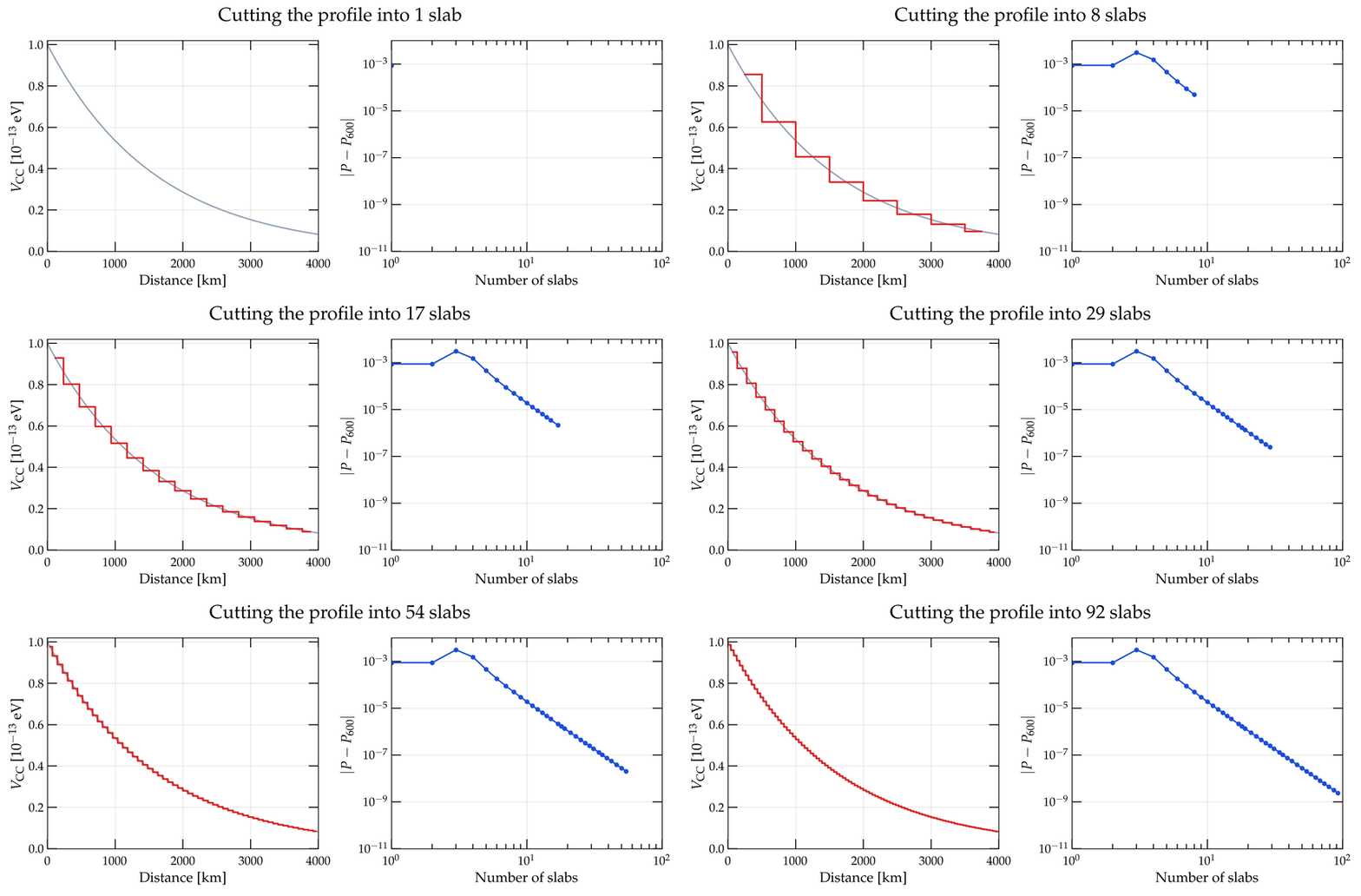
Two measurements make the difference concrete. On a smooth profile, multiplying constant-density slabs together bottoms out near 2.5 × 10⁻¹¹ and then gets worse: past roughly 16 000 slabs, round-off from composing that many matrix products outgrows anything a finer grid buys. Magνs keeps going to 2.9 × 10⁻¹³. And for the Sun, it returns 40 phase-averaged energies in about 0.7 s, where nuSQuIDS needs on the order of ten minutes merely to reach the solver tolerance at which its output is a probability at all.

The two packages deliberately share conventions, units and parameter defaults, so a calculation can be moved from one to the other and used as a cross-check on itself. I do this often.

Some physics it’s meant for

Each of these has a worked notebook in the tutorial gallery, and there is a systematic comparison against other codes in the documentation.

  • Long-baseline beams and atmospheric neutrinos through the Earth.
  • Solar neutrinos on a real tabulated model, including the averaged observable.
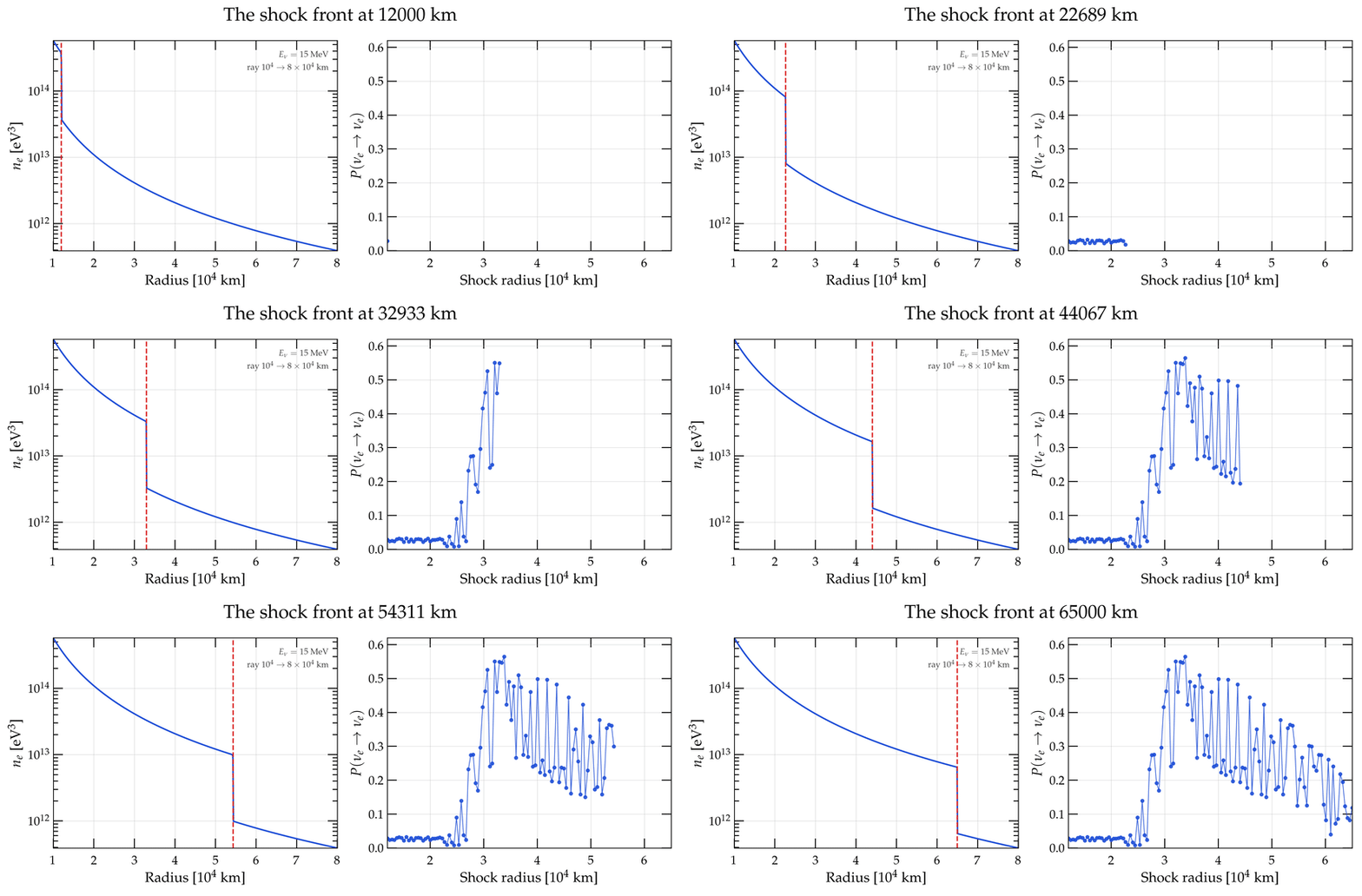
  • Supernova neutrinos across a shock front — where the width of the front is what decides which method the problem belongs to.
  • Sterile states (3+1 and 3+2), non-standard interactions, Lorentz-invariance violation.
  • A Hamiltonian of your own — the escape hatch, and the reason the rest of the list is not exhaustive.

NuOscProbExact 1.11.0: exact neutrino oscillation probabilities for two, three, and now four flavors — on PyPI!

Standard

Documentation: https://mbustama.github.io/NuOscProbExact/

Notebooks: https://github.com/mbustama/NuOscProbExact/tree/main/notebooks

Source code: https://github.com/mbustama/NuOscProbExact

PyPI: https://pypi.org/project/nuoscprobexact/

Neutrino oscillation probabilities look like a solved problem until the Hamiltonian stops being the textbook one. There is a closed form in vacuum, and another in two-flavor constant-density matter, and after that it runs out. Add a realistic density profile, a non-standard interaction, a Lorentz-violating operator or a fourth state, and the usual options are to expand in a parameter that may not be small, to diagonalise the Hamiltonian numerically at every point of a grid, or to integrate the Schrödinger equation and hope the step was short enough.

NuOscProbExact does none of these. The Hamiltonian and the time-evolution operator are expanded in the basis of SU(2), SU(3) or SU(4) matrices, and exponentiated analytically using the closure of the algebra. What comes out is a closed form for the probabilities in terms of two or three invariants of the Hamiltonian: no eigenvectors, no numerical diagonalisation, no integration, and no approximation beyond floating-point round-off. Any Hermitian 2×2, 3×3 or 4×4 matrix will do, whatever physics put it there. The method is Ohlsson and Snellman’s, revisited in the 2019 paper; the extension to SU(4) is new since then.

Four flavors is where it stops, for a reason external to neutrino physics: at five, the eigenvalues stop being expressible in radicals — Abel–Ruffini — and the closed form ends with them. Four is exactly what 3+1 needs.

If your reference point is a numerical evolution code, the output is the same object — probabilities, or the evolution operator itself — but with no step size to converge and no dependency beyond numpy. I wrote the first version because adding a model should mean writing down a matrix, not writing a solver. Seven years on it does rather more than it did, and version 1.11.0 now installs with pip.

What it makes easy

  • Any model, without a new code path. Vacuum, matter, non-standard interactions, Lorentz-invariance violation, sterile states: none of these is a special case in the code. Each is a different matrix handed to the same routine.
  • A whole scan in one call. A curve against energy or baseline, or a full oscillogram over both, with no Python loop.
  • Neutrinos through the Earth. Along a zenith angle, or between two of fifteen named sites — CERN–Gran Sasso, Fermilab–Homestake, Tokai–Kamioka and others — with the density profile taken from PREM. Or through any hand-built sequence of slabs of arbitrary width and density, each solved exactly and the operators multiplied.
  • 3+1 sterile scenarios at four flavors, as closed four-state systems rather than as leakage out of the three-flavor block.
  • The evolution operator itself, not only probabilities, for composing across segments or propagating a density matrix.

Install with:

pip install nuoscprobexact

and, for the optional compiled backend:

pip install "nuoscprobexact[fast]"

MIT licence. Python 3.9 or newer, tested on 3.9 through 3.13, and numpy is the only required dependency: no compiler, nothing to build.

Main features

Accuracy

  • Cross-checked against independently written code. The probabilities agree with nuSQuIDS to round-off once conventions are matched, and the matter spectrum agrees with the Zaglauer–Schwarzer closed form.
  • A regression suite of 596 tests, at 100% coverage.

Speed

  • Arrays instead of loops. Stacks of Hamiltonians, arrays of baselines, or both broadcast together: roughly 20x to 90x faster than the equivalent Python loop, with no extra dependency.
  • An optional compiled backend. With numba installed, the batched paths run as compiled kernels — answers identical to round-off, used only where it has been measured to win.

What you need to provide

You provide a Hermitian matrix and a baseline, built by hand or with one of the bundled builders for the standard cases. The package returns the exact evolution operator and the probabilities that follow from it, and stops there: no fluxes, no cross sections, no detector response, no fitting. One assumption is worth stating plainly: the Hamiltonian is taken to be time-independent over each segment. A smoothly varying profile can be slabbed, but the step size is then set by the oscillation rather than by the density, and there the documentation points at a Magnus-type method instead.

A minimal example

import numpy as np
import oscprob3nu
import hamiltonians3nu
from globaldefs import *
# The vacuum Hamiltonian, without the 1/E factor, so an energy scan
# computes it once
h_vac = hamiltonians3nu.hamiltonian_3nu_vacuum_energy_independent(
S12_NO_BF, S23_NO_BF, S13_NO_BF, DCP_NO_BF, D21_NO_BF, D31_NO_BF)
# One probability, at 1 GeV over 1300 km
Pee, Pem, Pet, Pme, Pmm, Pmt, Pte, Ptm, Ptt = oscprob3nu.probabilities_3nu(
np.asarray(h_vac)/1.e9, 1300.0*CONV_KM_TO_INV_EV)
print('Pee = %.5f, Pem = %.5f, Pet = %.5f' % (Pee, Pem, Pet))

prints

Pee = 0.92768, Pem = 0.01432, Pet = 0.05800


(The quickstart goes through this more slowly; the recipes page has short, complete snippets for most of what the package can compute, each with real output.)

What is new since 1.0.0

The original announcement, in May 2019, covered the method paper and the code on GitHub. The method has not changed since; almost everything around it has. Whole-array scans arrived in 1.2.0, the optional numba backend in 1.6.0, the Earth and arbitrary layered matter in 1.8.0, and four flavors — oscprob4nuhamiltonians4nu, the SU(4) expansion — in 1.9.0. In 1.11.0, a non-Hermitian Hamiltonian raises instead of quietly returning probabilities that still sum to one. Along the way, a documentation site and eighteen worked notebooks.

One thing to flag for anyone still running 1.0.0: two fixes in 1.1.0 changed numbers, both at two flavors. probabilities_2nu was missing the h2 contribution to P(νe → νμ), which is invisible whenever the off-diagonal entry is real — so vacuum and constant-density matter were unaffected, but a CP-violating two-flavor Hamiltonian was not — and the two-flavor vacuum Hamiltonian used the opposite sign convention, invisible in vacuum and consequential once a matter potential is added. Three-flavor results from 1.0.0 are unaffected; the changelog has the details.

Some physics it’s meant for

Long-baseline accelerator experiments. DUNE-like baselines through the crust, with matter effects and the CP phase, and the bi-probability ellipses above, which show how matter pushes neutrinos and antineutrinos off the CP-symmetric diagonal. Notebook 05.

Atmospheric neutrinos through the Earth. Zenith-angle scans with the density taken from PREM rather than from a single average value, which is where the mass ordering and the θ23 octant separate. Notebooks 07 and 12.

Sterile neutrinos, 3+1. Short-baseline appearance and disappearance, and the sterile matter resonance through the Earth, with the four states treated as a closed, unitary system rather than as leakage out of the three-flavor block. Notebook 16.

Non-standard interactions and Lorentz-invariance violation. Both enter as extra Hermitian terms added to the vacuum Hamiltonian, so a new operator means a new matrix, not a new solver. Notebook 03.

Unusual matter profiles. Castle-wall and other hand-built profiles, where the arrangement of the matter changes the answer even when the mean density does not — a parametric-resonance effect no constant-density approximation can show. Notebook 08.

Wrap-up of the 2025 NBI Neutrino School

Standard

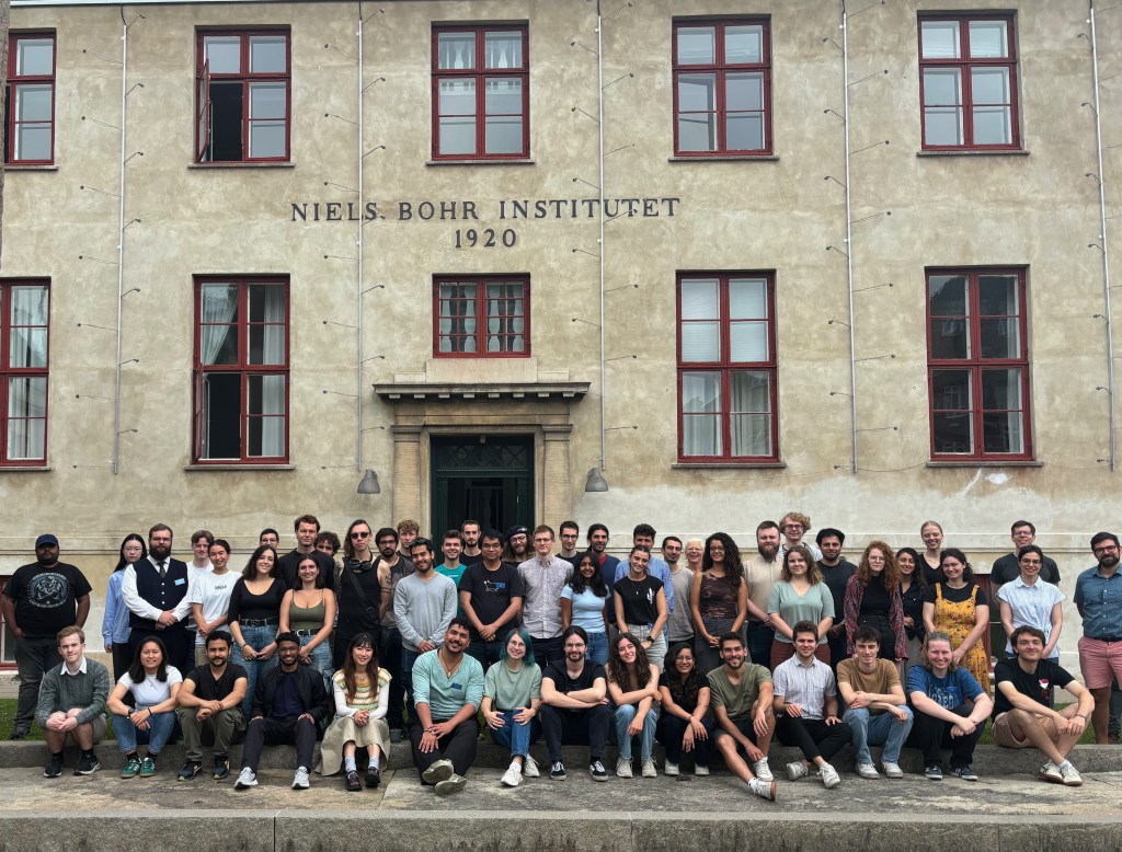
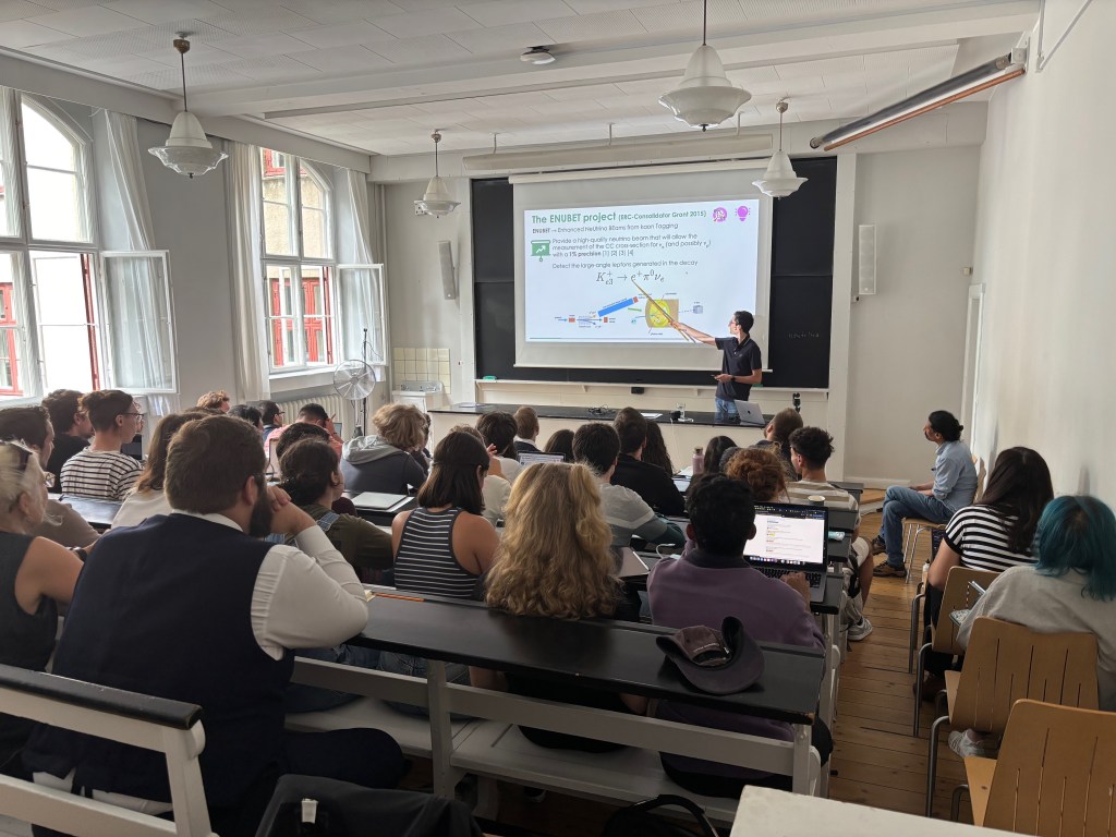
The IV NBI PhD Summer School on Neutrinos has wrapped!

From July 7 to 11, 2025, we hosted 53 PhD, MSc, and BSc students from around the world. They received lectures on neutrino theory & phenomenology, neutrino astrophysics, and neutrino cosmology. All in all, we had 9 lectures, 5 topical seminars from NBI locals, and 24 student talks.

Here are a few photos (photo credit to co-organizer Markus Ahlers):

Like for the 2021, 2022, and 2023 schools, all the videos from the school are available on our YouTube channel.

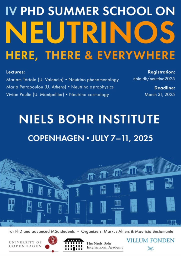
IV NBI Neutrino Summer School “Here, There & Everywhere”

Standard

Registration is now open for the fourth edition of our NBI Neutrino Summer School, “Here, There & Everywhere”.

Like in previous editions (2021, 2022, 2023), the school is aimed at PhD students and advanced MSc students from all over the world that work on neutrinos, are planning to work on them, or are simply interested in them! The school is a one-week series of lectures on neutrino phenomenology, astrophysics, and cosmology delivered by carefully chosen world experts on these subjects.

When? July 7-11, 2025

Where? Niels Bohr Institute, Copenhagen, Denmark

How to register? Go to our Indico page here

Registration deadline: March 31, 2025 (register early!)

Can you present a student talk? Accepted in-person participants are encouraged to submit an abstract

Is there a participation fee? Yes, there is a fee of 130 EUR for in-person participants

Questions? Find our contact information (Markus Ahlers, Mauricio Bustamante) on the Indico page

The school provides lunch (Monday to Friday), two coffee breaks a days, reception and a school dinner.

Discovering Majorons from the neutrinos of the next galactic supernova

Standard

In the hot, dense cores of core-collapse supernova, neutrinos could coalesce to make new, heavy particles, like Majoron-like bosons, with masses from tens of MeV to more than 100 MeV. After escaping the supernova, these Majorons would decay into energies comparable to the parent Majoron mass, far more energetic than the standard supernova neutrinos emitted from the neutrinosphere, and arriving at Earth later than them.

Thanks to large upcoming neutrino detectors, we might observe these high-energy neutrinos from the next galactic core-collapse supernova. Combining all available detection channels provides us with information on the energy, flavor, and arrival times of these neutrinos.

In a new paper, led by NBI PhD student Bernanda Telalovic, we have shown for the first time that we can combine this information use to clearly distinguish neutrinos from Majoron decay from the standard neutrinos of the next galactic supernova.

And, on top of that, we fold in the large uncertainty that exists in supernova physics by using two sophisticated supernova simulations (hot and cold) from the Garching group, obtained for two different assumptions for the mass of the proto-neutron star. However, our results do not hinge on us knowing what the real model, since we marginalize over it.

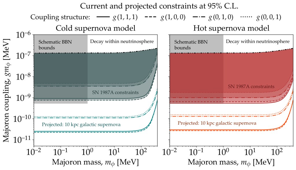
Should we detect no high-energy neutrinos, we will be able to place upper bounds on the Majoron coupling to neutrinos that are more than an order of magnitude stronger than the ones inferred from the observation of neutrinos from SN 1987A:

We show explicitly how the bounds are different depending on the flavor texture of the Majoron.

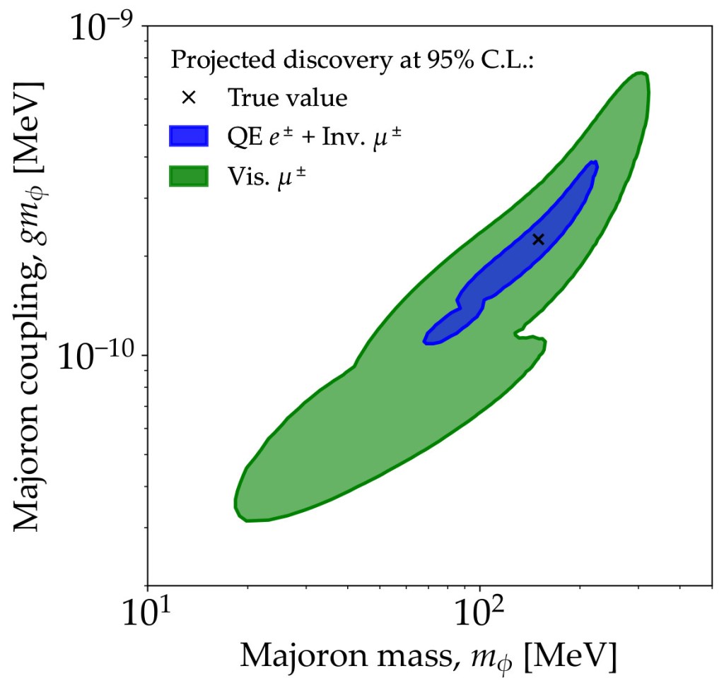
Conversely, should we detect high-energy neutrinos with late arrival times (tens of seconds post-bounce), we will be able to measure the mass and flavor-universal coupling of the Majoron:

Read more at:

The next galactic supernova can uncover mass and couplings of particles decaying to neutrinos
Bernanda Telalovic, Damiano F.G. Fiorillo, Pablo Martíinez-Miravé, Edoardo Vitagliano, Mauricio Bustamante
2406.15506 astro-ph