Documentation: https://mbustama.github.io/NuOscProbExact/
Notebooks: https://github.com/mbustama/NuOscProbExact/tree/main/notebooks
Source code: https://github.com/mbustama/NuOscProbExact
PyPI: https://pypi.org/project/nuoscprobexact/
Neutrino oscillation probabilities look like a solved problem until the Hamiltonian stops being the textbook one. There is a closed form in vacuum, and another in two-flavor constant-density matter, and after that it runs out. Add a realistic density profile, a non-standard interaction, a Lorentz-violating operator or a fourth state, and the usual options are to expand in a parameter that may not be small, to diagonalise the Hamiltonian numerically at every point of a grid, or to integrate the Schrödinger equation and hope the step was short enough.
NuOscProbExact does none of these. The Hamiltonian and the time-evolution operator are expanded in the basis of SU(2), SU(3) or SU(4) matrices, and exponentiated analytically using the closure of the algebra. What comes out is a closed form for the probabilities in terms of two or three invariants of the Hamiltonian: no eigenvectors, no numerical diagonalisation, no integration, and no approximation beyond floating-point round-off. Any Hermitian 2×2, 3×3 or 4×4 matrix will do, whatever physics put it there. The method is Ohlsson and Snellman’s, revisited in the 2019 paper; the extension to SU(4) is new since then.
Four flavors is where it stops, for a reason external to neutrino physics: at five, the eigenvalues stop being expressible in radicals — Abel–Ruffini — and the closed form ends with them. Four is exactly what 3+1 needs.
If your reference point is a numerical evolution code, the output is the same object — probabilities, or the evolution operator itself — but with no step size to converge and no dependency beyond numpy. I wrote the first version because adding a model should mean writing down a matrix, not writing a solver. Seven years on it does rather more than it did, and version 1.11.0 now installs with pip.
What it makes easy
- Any model, without a new code path. Vacuum, matter, non-standard interactions, Lorentz-invariance violation, sterile states: none of these is a special case in the code. Each is a different matrix handed to the same routine.
- A whole scan in one call. A curve against energy or baseline, or a full oscillogram over both, with no Python loop.
- Neutrinos through the Earth. Along a zenith angle, or between two of fifteen named sites — CERN–Gran Sasso, Fermilab–Homestake, Tokai–Kamioka and others — with the density profile taken from PREM. Or through any hand-built sequence of slabs of arbitrary width and density, each solved exactly and the operators multiplied.
- 3+1 sterile scenarios at four flavors, as closed four-state systems rather than as leakage out of the three-flavor block.
- The evolution operator itself, not only probabilities, for composing across segments or propagating a density matrix.
Install with:
and, for the optional compiled backend:
MIT licence. Python 3.9 or newer, tested on 3.9 through 3.13, and numpy is the only required dependency: no compiler, nothing to build.
Main features
Accuracy
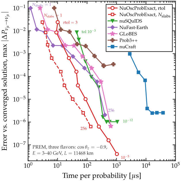
- Cross-checked against independently written code. The probabilities agree with nuSQuIDS to round-off once conventions are matched, and the matter spectrum agrees with the Zaglauer–Schwarzer closed form.
- A regression suite of 596 tests, at 100% coverage.
Speed
- Arrays instead of loops. Stacks of Hamiltonians, arrays of baselines, or both broadcast together: roughly 20x to 90x faster than the equivalent Python loop, with no extra dependency.
- An optional compiled backend. With
numba installed, the batched paths run as compiled kernels — answers identical to round-off, used only where it has been measured to win.
What you need to provide
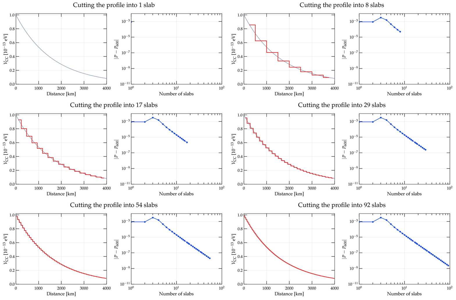
You provide a Hermitian matrix and a baseline, built by hand or with one of the bundled builders for the standard cases. The package returns the exact evolution operator and the probabilities that follow from it, and stops there: no fluxes, no cross sections, no detector response, no fitting. One assumption is worth stating plainly: the Hamiltonian is taken to be time-independent over each segment. A smoothly varying profile can be slabbed, but the step size is then set by the oscillation rather than by the density, and there the documentation points at a Magnus-type method instead.
A minimal example
prints
(The quickstart goes through this more slowly; the recipes page has short, complete snippets for most of what the package can compute, each with real output.)
What is new since 1.0.0
The original announcement, in May 2019, covered the method paper and the code on GitHub. The method has not changed since; almost everything around it has. Whole-array scans arrived in 1.2.0, the optional numba backend in 1.6.0, the Earth and arbitrary layered matter in 1.8.0, and four flavors — oscprob4nu, hamiltonians4nu, the SU(4) expansion — in 1.9.0. In 1.11.0, a non-Hermitian Hamiltonian raises instead of quietly returning probabilities that still sum to one. Along the way, a documentation site and eighteen worked notebooks.
One thing to flag for anyone still running 1.0.0: two fixes in 1.1.0 changed numbers, both at two flavors. probabilities_2nu was missing the h2 contribution to P(νe → νμ), which is invisible whenever the off-diagonal entry is real — so vacuum and constant-density matter were unaffected, but a CP-violating two-flavor Hamiltonian was not — and the two-flavor vacuum Hamiltonian used the opposite sign convention, invisible in vacuum and consequential once a matter potential is added. Three-flavor results from 1.0.0 are unaffected; the changelog has the details.
Some physics it’s meant for
Long-baseline accelerator experiments. DUNE-like baselines through the crust, with matter effects and the CP phase, and the bi-probability ellipses above, which show how matter pushes neutrinos and antineutrinos off the CP-symmetric diagonal. Notebook 05.
Atmospheric neutrinos through the Earth. Zenith-angle scans with the density taken from PREM rather than from a single average value, which is where the mass ordering and the θ23 octant separate. Notebooks 07 and 12.
Sterile neutrinos, 3+1. Short-baseline appearance and disappearance, and the sterile matter resonance through the Earth, with the four states treated as a closed, unitary system rather than as leakage out of the three-flavor block. Notebook 16.
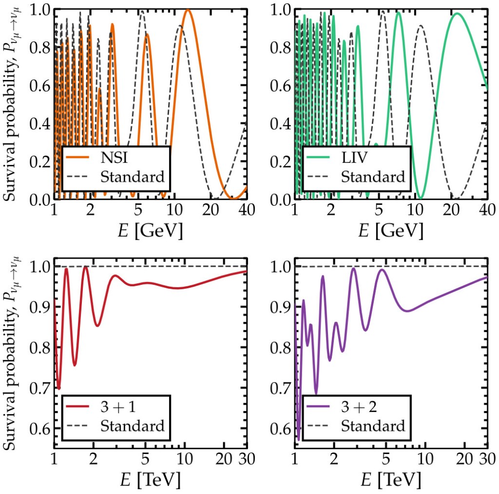
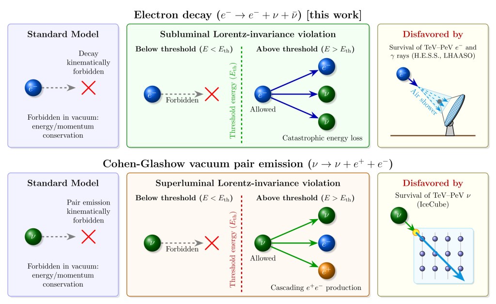
Non-standard interactions and Lorentz-invariance violation. Both enter as extra Hermitian terms added to the vacuum Hamiltonian, so a new operator means a new matrix, not a new solver. Notebook 03.
Unusual matter profiles. Castle-wall and other hand-built profiles, where the arrangement of the matter changes the answer even when the mean density does not — a parametric-resonance effect no constant-density approximation can show. Notebook 08.