Magnus: neutrino oscillation probabilities for any Hamiltonian, in any number of flavors

Documentation: https://mbustama.github.io/Magnus/

Notebooks: https://mbustama.github.io/Magnus/tutorials.html

Source code: https://github.com/mbustama/Magnus

PyPI: https://pypi.org/project/magnuspy/

Oscillations in matter are usually computed by pretending the matter holds still: chop the path into slabs of constant density, solve each one exactly, multiply. It is a good trick, and for a neutrino crossing the Earth it is nearly the truth. For the Sun, for a supernova, for anything with a front moving through it, the pretending is where the physics is.

Magνs is my new package for that case. It computes oscillation probabilities for an arbitrary number of flavors, under any Hamiltonian, whether or not it depends on time. Rather than stepping the Schrödinger equation forward, it integrates the Hamiltonian across each slab and exponentiates the result — the Magnus expansion. The useful consequence is structural: however hard the expansion is truncated, the truncation stays inside the Lie algebra, so the evolution operator is exactly unitary by construction. Probabilities come out non-negative and summing to one at machine precision, at every accuracy setting, not only the expensive ones.

What it makes easy

A density that actually changes — a tabulated solar model, a supernova profile from a simulation, a shock front.
An accuracy instead of a slab count — ask for a tolerance and the refinement finds the resolution for you.
Any number of flavors — two through five, sterile states (3+1, 3+2) included.
The phase-averaged probability, in closed form — the quantity a solar experiment actually measures, returned directly rather than reconstructed by averaging a scan.
Neutrinos through the Earth — you give a direction, not a profile.

Install with:

pip install magnuspy

The import package is magnus. Python 3.10 or newer, GPL-3.0-only, and 27 example notebooks that are executed in CI, so the numbers printed in them cannot quietly drift.

A minimal example

A 10 GeV muon neutrino arriving from below, crossing the Earth:

			
import magnus.oscprob as oscprob
import magnus.globaldefs as gd
import magnus.earth as earth
# A 10 GeV muon neutrino crossing the Earth, arriving from below.
costhz = -0.4
L = earth.distance_traveled_inside_earth(costhz)*gd.UNIT_KM   # chord: km -> eV^-1
P = oscprob.osc_prob_3nu_earth(10.0*gd.UNIT_GEV, costhz=costhz, L=L)
print('Pme = %.5f, Pmm = %.5f, Pmt = %.5f'
      % (P[gd.NUMU][gd.NUE], P[gd.NUMU][gd.NUMU], P[gd.NUMU][gd.NUTAU]))

		

which prints

Pme = 0.10273, Pmm = 0.01165, Pmt = 0.88562

The oscillation parameters are never mentioned, because they default to the current global fit (NuFIT 6.1). Neither is the Earth’s density: the wrapper walks the PREM profile for the chord that the zenith angle picks out. What you supply is a direction and an energy.

How it differs from NuOscProbExact

Both packages are mine, and they are not competitors — the honest way to put it is as a boundary rather than a winner. NuOscProbExact solves each constant-density slab in closed form, through SU(2), SU(3) and SU(4) expansions. It is exact up to round-off, there is no slab count to argue about, and it is fast. Where a closed form exists and the accumulated phase is large, use the closed form — including the Earth through PREM at three flavors, where NuOscProbExact is about 20× cheaper per call than Magνs. That is its home ground.

Magνs integrates across each slab instead, which is exactly what lets it follow a density that changes while the neutrino is still inside it. Reach for it when the profile varies continuously, when you would rather ask for an accuracy than guess a resolution, when you need five flavors — the SU(N) closed forms stop at SU(4) — or when the Hamiltonian is something nobody has diagonalized.

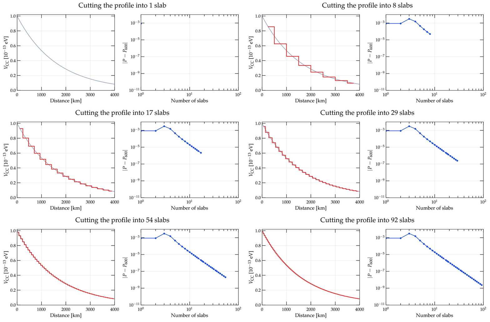
Two measurements make the difference concrete. On a smooth profile, multiplying constant-density slabs together bottoms out near 2.5 × 10⁻¹¹ and then gets worse: past roughly 16 000 slabs, round-off from composing that many matrix products outgrows anything a finer grid buys. Magνs keeps going to 2.9 × 10⁻¹³. And for the Sun, it returns 40 phase-averaged energies in about 0.7 s, where nuSQuIDS needs on the order of ten minutes merely to reach the solver tolerance at which its output is a probability at all.

The two packages deliberately share conventions, units and parameter defaults, so a calculation can be moved from one to the other and used as a cross-check on itself. I do this often.

Some physics it’s meant for

Each of these has a worked notebook in the tutorial gallery, and there is a systematic comparison against other codes in the documentation.

Long-baseline beams and atmospheric neutrinos through the Earth.
Solar neutrinos on a real tabulated model, including the averaged observable.
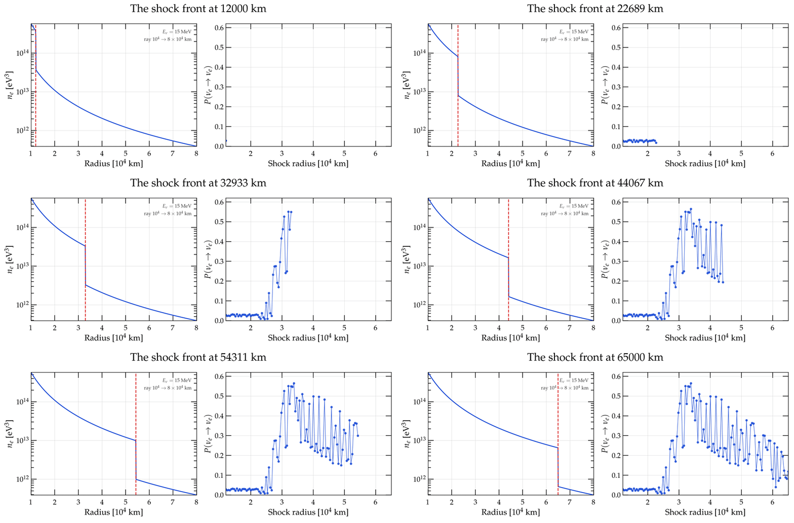
Supernova neutrinos across a shock front — where the width of the front is what decides which method the problem belongs to.
Sterile states (3+1 and 3+2), non-standard interactions, Lorentz-invariance violation.
A Hamiltonian of your own — the escape hatch, and the reason the rest of the list is not exhaustive.

Electron stability constrains neutrino time delays

The search for Lorentz-invariance violation (LIV) is one of our best paths toward uncovering the quantum nature of spacetime. One of its most famous potential manifestations is the modification of neutrino propagation speeds.

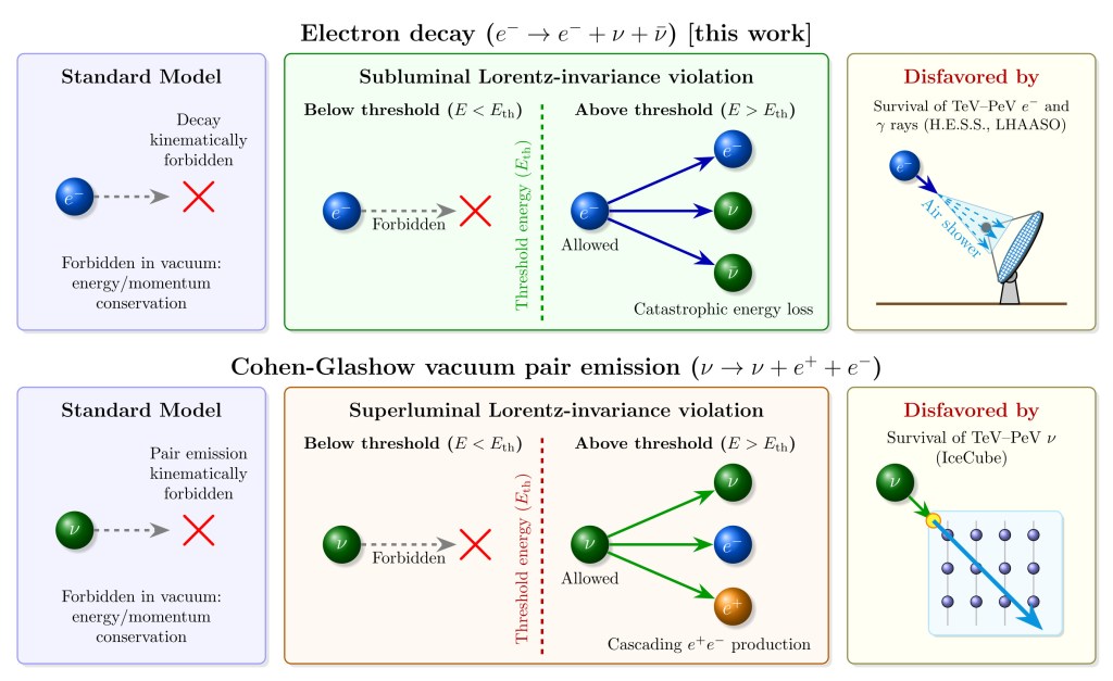
For years, the community has known that superluminal (faster-than-light) neutrinos are heavily constrained. LIV would cause them to rapidly lose energy by radiating electron-positron pairs in a vacuum. Because of this, when anomalous time delays between cosmic neutrinos and gamma rays are observed, phenomenologists have naturally favored subluminal (slower-than-light) LIV propagation as the most viable explanation.

In a new paper co-authored with José Manuel Carmona, José Luis Cortés, Ardit Gkioni, and Maykoll A. Reyes, we demonstrate that this apparent subluminal loophole is actually an illusion.

We show that the same LIV modifications that slow down neutrinos inevitably render high-energy electrons unstable. Under subluminal LIV, electrons undergo a catastrophic decay process: e⁻ → e⁻ + ν + anti-ν. This triggers rapid and severe energy degradation.

By demanding that electrons survive up to the extreme energies we observe in astrophysics—specifically, the 15.5-TeV candidates from H.E.S.S. and the 2.34-PeV electrons inferred by LHAASO in the Crab Nebula—we placed stringent new limits on subluminal LIV.

Our results firmly invalidate the subluminal parameter space previously invoked to explain years-long cosmic neutrino time delays. Consequently, any observable delays must either have purely astrophysical origins, rely on a universal LIV deformation across all particle species, or require physics well beyond the standard effective-field-theory framework.

Read more at:

Electron stability constrains neutrino time delays
Mauricio Bustamante, José Manuel Carmona, José Luis Cortés, Ardit Gkioni, Maykoll A. Reyes
2607.01339 hep-ph

No Flavor Anisotropy in the High-Energy Neutrino Sky Upholds Lorentz Invariance

Do neutrinos of different flavors have different preferred directions? If so, this would mean that Lorentz invariance is violated, something that is posited by some theories of quantum gravity. In them, Lorentz-invariance violation (LIV) would become more prominent the higher the energies involved.

Motivated by this, we look for signs of this flavor-dependent LIV using the high-energy astrophysical neutrinos seen by IceCube, with energies in the TeV-PeV range.

If LIV exists, the neutrinos would be affected by their interaction with a pervasive LIV field that couples differently to different neutrino flavors. As a result, the sky distributions of high-energy astrophysical electron, muon, and tau neutrinos arriving at Earth would be anisotropic.

In a new paper led by PhD student Bernanda Telalovic, we look for these high-energy neutrino flavor anisotropies in IceCube data, specifically, in the public 7.5-year sample of High-Energy Starting Events (HESE). We do this using the methods introduced in an earlier paper of ours (2310.15224).

We find no evidence for the patterns of flavor anisotropy expected from LIV, and so we place new upper limits on hundreds of parameters regulating Lorentz-invariance violation within the Standard Model Extension. We explore LIV operator dimensions from 2 to 8, each with a different dependence on neutrino energy and introducing different forms of flavor anisotropy.

For many of them, we improve upon existing limits—on account of using higher energies—or place limits for the first time ever:

Our new upper limits on the LIV parameters are available in digital form for download at 68%, 95%, and 99% C.L. GitHub, here.

Testing Lorentz invariance with a flare of high-energy astrophysical neutrinos

Lorentz invariance is one of the pillars of modern physics, underlying special relativity—and, with that, the Standard Model—and general relativity. It posits that the laws of physics are the same for all observers moving in their own inertial frame. Yet, at high energies and short distances, Lorentz invariance may no longer hold.

To date, Lorentz invariance remains unbroken in all experimental tests. If it were violated, however, it could have many and varied consequences. Accordingly, there have been multiple searches for Lorentz invariance violation, using atom interferometry, gamma rays, cosmic rays, and neutrinos, etc. See, for instance, the data tables in 0801.0287.

High-energy astrophysical neutrinos, with TeV-PeV, are powerful probes of Lorentz invariance, thanks to their high energies and long traveled distances from their sources to Earth, of Mpc-Gpc scales. If Lorentz invariance is violated, it could imply that, en route to Earth, higher-energy neutrinos would travel more slowly than lower-energy neutrinos.

In a new paper, we introduce methods to look for these temporal distortions. We use the high-energy joint time and energy distribution of the neutrino flare detected by IceCube in 2014/2015 from the blazar TXS 0506+056 to look for specific signatures from Lorentz-invariance violation. We do this by borrowing non-parametric statistical methods previously used to look for signs of Lorentz-invariance violation in the gamma rays from gamma-ray bursts (1807.00189).

And, in doing so, we account for the significant energy and directional uncertainty associated to the detection of high-energy astrophysical neutrinos. Doing this makes our analysis realistic and robust, even if it erodes some of its sensitivity.

As a result, we set new lower limits on the energy scale of Lorentz-invariance violation in neutrino propagation. If Lorentz invariance is broken, this must happen at energies beyond 10^{14} GeV, if the effects depend linearly on the neutrino energy, or beyond 10^9 GeV, if they depend quadratically on it.

Mauricio Bustamante

Associate Professor – Niels Bohr Institute, University of Copenhagen

lorentz