

Documentation: https://mbustama.github.io/Magnus/
Notebooks: https://mbustama.github.io/Magnus/tutorials.html
Source code: https://github.com/mbustama/Magnus
PyPI: https://pypi.org/project/magnuspy/
Oscillations in matter are usually computed by pretending the matter holds still: chop the path into slabs of constant density, solve each one exactly, multiply. It is a good trick, and for a neutrino crossing the Earth it is nearly the truth. For the Sun, for a supernova, for anything with a front moving through it, the pretending is where the physics is.
Magνs is my new package for that case. It computes oscillation probabilities for an arbitrary number of flavors, under any Hamiltonian, whether or not it depends on time. Rather than stepping the Schrödinger equation forward, it integrates the Hamiltonian across each slab and exponentiates the result — the Magnus expansion. The useful consequence is structural: however hard the expansion is truncated, the truncation stays inside the Lie algebra, so the evolution operator is exactly unitary by construction. Probabilities come out non-negative and summing to one at machine precision, at every accuracy setting, not only the expensive ones.
What it makes easy
- A density that actually changes — a tabulated solar model, a supernova profile from a simulation, a shock front.
- An accuracy instead of a slab count — ask for a tolerance and the refinement finds the resolution for you.
- Any number of flavors — two through five, sterile states (3+1, 3+2) included.
- The phase-averaged probability, in closed form — the quantity a solar experiment actually measures, returned directly rather than reconstructed by averaging a scan.
- Neutrinos through the Earth — you give a direction, not a profile.
Install with:
pip install magnuspy
The import package is magnus. Python 3.10 or newer, GPL-3.0-only, and 27 example notebooks that are executed in CI, so the numbers printed in them cannot quietly drift.
A minimal example
A 10 GeV muon neutrino arriving from below, crossing the Earth:
import magnus.oscprob as oscprobimport magnus.globaldefs as gdimport magnus.earth as earth# A 10 GeV muon neutrino crossing the Earth, arriving from below.costhz = -0.4L = earth.distance_traveled_inside_earth(costhz)*gd.UNIT_KM # chord: km -> eV^-1P = oscprob.osc_prob_3nu_earth(10.0*gd.UNIT_GEV, costhz=costhz, L=L)print('Pme = %.5f, Pmm = %.5f, Pmt = %.5f' % (P[gd.NUMU][gd.NUE], P[gd.NUMU][gd.NUMU], P[gd.NUMU][gd.NUTAU]))
which prints
Pme = 0.10273, Pmm = 0.01165, Pmt = 0.88562
The oscillation parameters are never mentioned, because they default to the current global fit (NuFIT 6.1). Neither is the Earth’s density: the wrapper walks the PREM profile for the chord that the zenith angle picks out. What you supply is a direction and an energy.

How it differs from NuOscProbExact
Both packages are mine, and they are not competitors — the honest way to put it is as a boundary rather than a winner. NuOscProbExact solves each constant-density slab in closed form, through SU(2), SU(3) and SU(4) expansions. It is exact up to round-off, there is no slab count to argue about, and it is fast. Where a closed form exists and the accumulated phase is large, use the closed form — including the Earth through PREM at three flavors, where NuOscProbExact is about 20× cheaper per call than Magνs. That is its home ground.
Magνs integrates across each slab instead, which is exactly what lets it follow a density that changes while the neutrino is still inside it. Reach for it when the profile varies continuously, when you would rather ask for an accuracy than guess a resolution, when you need five flavors — the SU(N) closed forms stop at SU(4) — or when the Hamiltonian is something nobody has diagonalized.
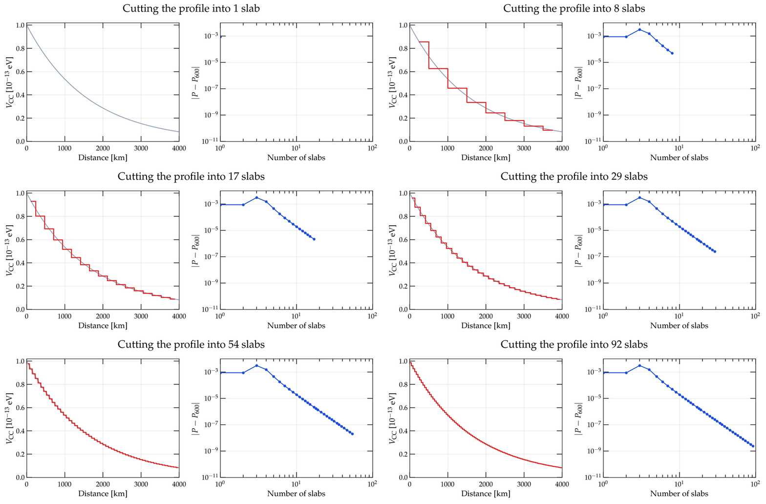
Two measurements make the difference concrete. On a smooth profile, multiplying constant-density slabs together bottoms out near 2.5 × 10⁻¹¹ and then gets worse: past roughly 16 000 slabs, round-off from composing that many matrix products outgrows anything a finer grid buys. Magνs keeps going to 2.9 × 10⁻¹³. And for the Sun, it returns 40 phase-averaged energies in about 0.7 s, where nuSQuIDS needs on the order of ten minutes merely to reach the solver tolerance at which its output is a probability at all.
The two packages deliberately share conventions, units and parameter defaults, so a calculation can be moved from one to the other and used as a cross-check on itself. I do this often.

Some physics it’s meant for
Each of these has a worked notebook in the tutorial gallery, and there is a systematic comparison against other codes in the documentation.
- Long-baseline beams and atmospheric neutrinos through the Earth.
- Solar neutrinos on a real tabulated model, including the averaged observable.
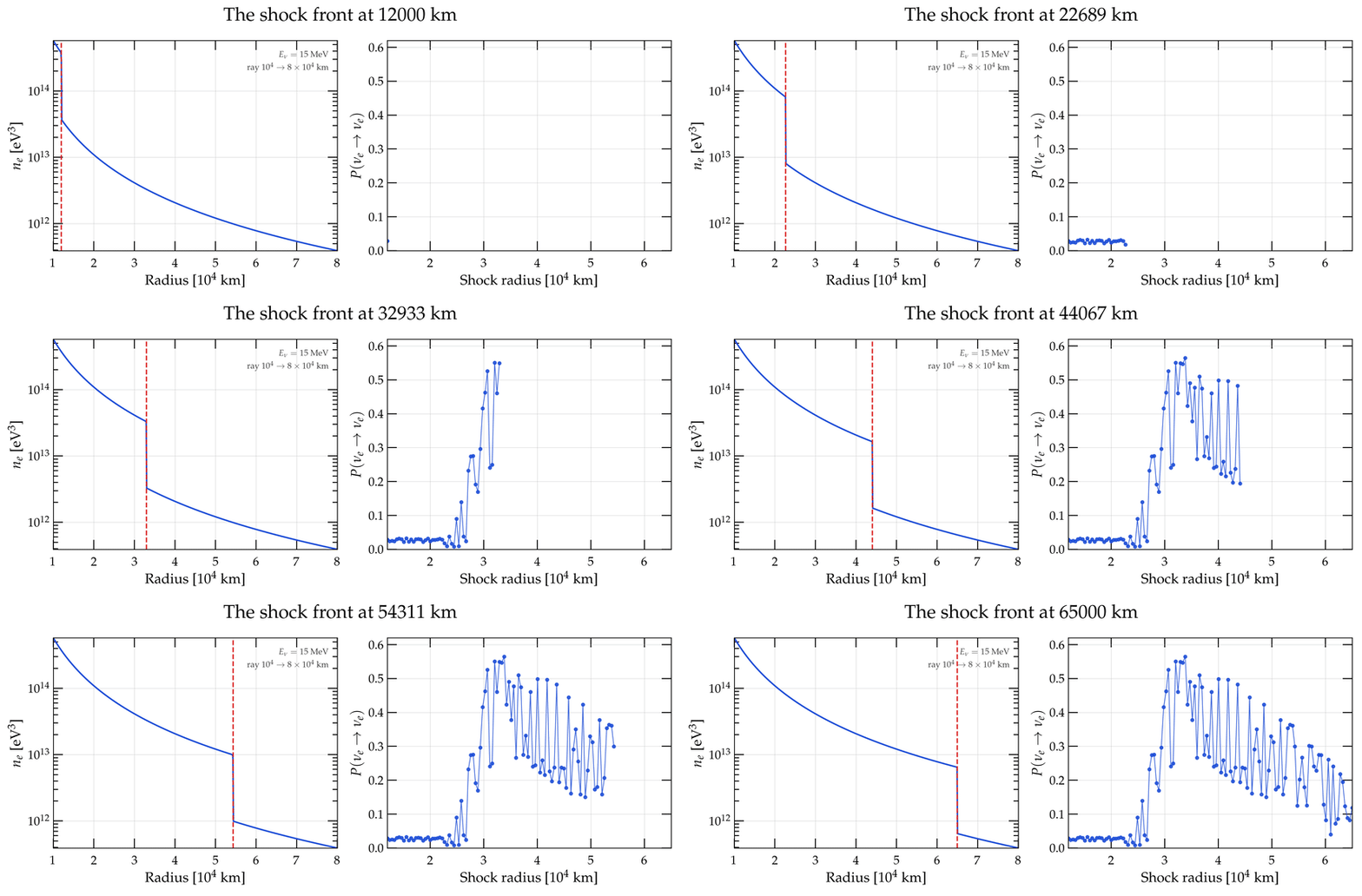
- Supernova neutrinos across a shock front — where the width of the front is what decides which method the problem belongs to.
- Sterile states (3+1 and 3+2), non-standard interactions, Lorentz-invariance violation.
- A Hamiltonian of your own — the escape hatch, and the reason the rest of the list is not exhaustive.

