Interview in PuntoEdu (PUCP) — August 21, 2026

PuntoEdu, the institutional magazine of my alma mater, the Pontificia Universidad Católica del Perú, interviewed me about my recent appointment as co-spokesperson of GRAND, together with Zhang Yi (Purple Mountain Observatory, Nanjing). We also talked about TAMBO, the high-energy tau-neutrino observatory proposed for the Colca Valley in Arequipa; about using astrophysical neutrinos to look for physics beyond the Standard Model; and about what my undergraduate and MSc years at PUCP left me with — above all, the habit of doubting my own results first. The headline quote translates as “PUCP gives you the chance to do international-level science while staying more or less at home.”

Interview by Gabriela Machuca Castillo.

Note: the interview is in Spanish.

Read it here →

Magnus: neutrino oscillation probabilities for any Hamiltonian, in any number of flavors

Documentation: https://mbustama.github.io/Magnus/

Notebooks: https://mbustama.github.io/Magnus/tutorials.html

Source code: https://github.com/mbustama/Magnus

PyPI: https://pypi.org/project/magnuspy/

Oscillations in matter are usually computed by pretending the matter holds still: chop the path into slabs of constant density, solve each one exactly, multiply. It is a good trick, and for a neutrino crossing the Earth it is nearly the truth. For the Sun, for a supernova, for anything with a front moving through it, the pretending is where the physics is.

Magνs is my new package for that case. It computes oscillation probabilities for an arbitrary number of flavors, under any Hamiltonian, whether or not it depends on time. Rather than stepping the Schrödinger equation forward, it integrates the Hamiltonian across each slab and exponentiates the result — the Magnus expansion. The useful consequence is structural: however hard the expansion is truncated, the truncation stays inside the Lie algebra, so the evolution operator is exactly unitary by construction. Probabilities come out non-negative and summing to one at machine precision, at every accuracy setting, not only the expensive ones.

What it makes easy

A density that actually changes — a tabulated solar model, a supernova profile from a simulation, a shock front.
An accuracy instead of a slab count — ask for a tolerance and the refinement finds the resolution for you.
Any number of flavors — two through five, sterile states (3+1, 3+2) included.
The phase-averaged probability, in closed form — the quantity a solar experiment actually measures, returned directly rather than reconstructed by averaging a scan.
Neutrinos through the Earth — you give a direction, not a profile.

Install with:

pip install magnuspy

The import package is magnus. Python 3.10 or newer, GPL-3.0-only, and 27 example notebooks that are executed in CI, so the numbers printed in them cannot quietly drift.

A minimal example

A 10 GeV muon neutrino arriving from below, crossing the Earth:

			
import magnus.oscprob as oscprob
import magnus.globaldefs as gd
import magnus.earth as earth
# A 10 GeV muon neutrino crossing the Earth, arriving from below.
costhz = -0.4
L = earth.distance_traveled_inside_earth(costhz)*gd.UNIT_KM   # chord: km -> eV^-1
P = oscprob.osc_prob_3nu_earth(10.0*gd.UNIT_GEV, costhz=costhz, L=L)
print('Pme = %.5f, Pmm = %.5f, Pmt = %.5f'
      % (P[gd.NUMU][gd.NUE], P[gd.NUMU][gd.NUMU], P[gd.NUMU][gd.NUTAU]))

		

which prints

Pme = 0.10273, Pmm = 0.01165, Pmt = 0.88562

The oscillation parameters are never mentioned, because they default to the current global fit (NuFIT 6.1). Neither is the Earth’s density: the wrapper walks the PREM profile for the chord that the zenith angle picks out. What you supply is a direction and an energy.

How it differs from NuOscProbExact

Both packages are mine, and they are not competitors — the honest way to put it is as a boundary rather than a winner. NuOscProbExact solves each constant-density slab in closed form, through SU(2), SU(3) and SU(4) expansions. It is exact up to round-off, there is no slab count to argue about, and it is fast. Where a closed form exists and the accumulated phase is large, use the closed form — including the Earth through PREM at three flavors, where NuOscProbExact is about 20× cheaper per call than Magνs. That is its home ground.

Magνs integrates across each slab instead, which is exactly what lets it follow a density that changes while the neutrino is still inside it. Reach for it when the profile varies continuously, when you would rather ask for an accuracy than guess a resolution, when you need five flavors — the SU(N) closed forms stop at SU(4) — or when the Hamiltonian is something nobody has diagonalized.

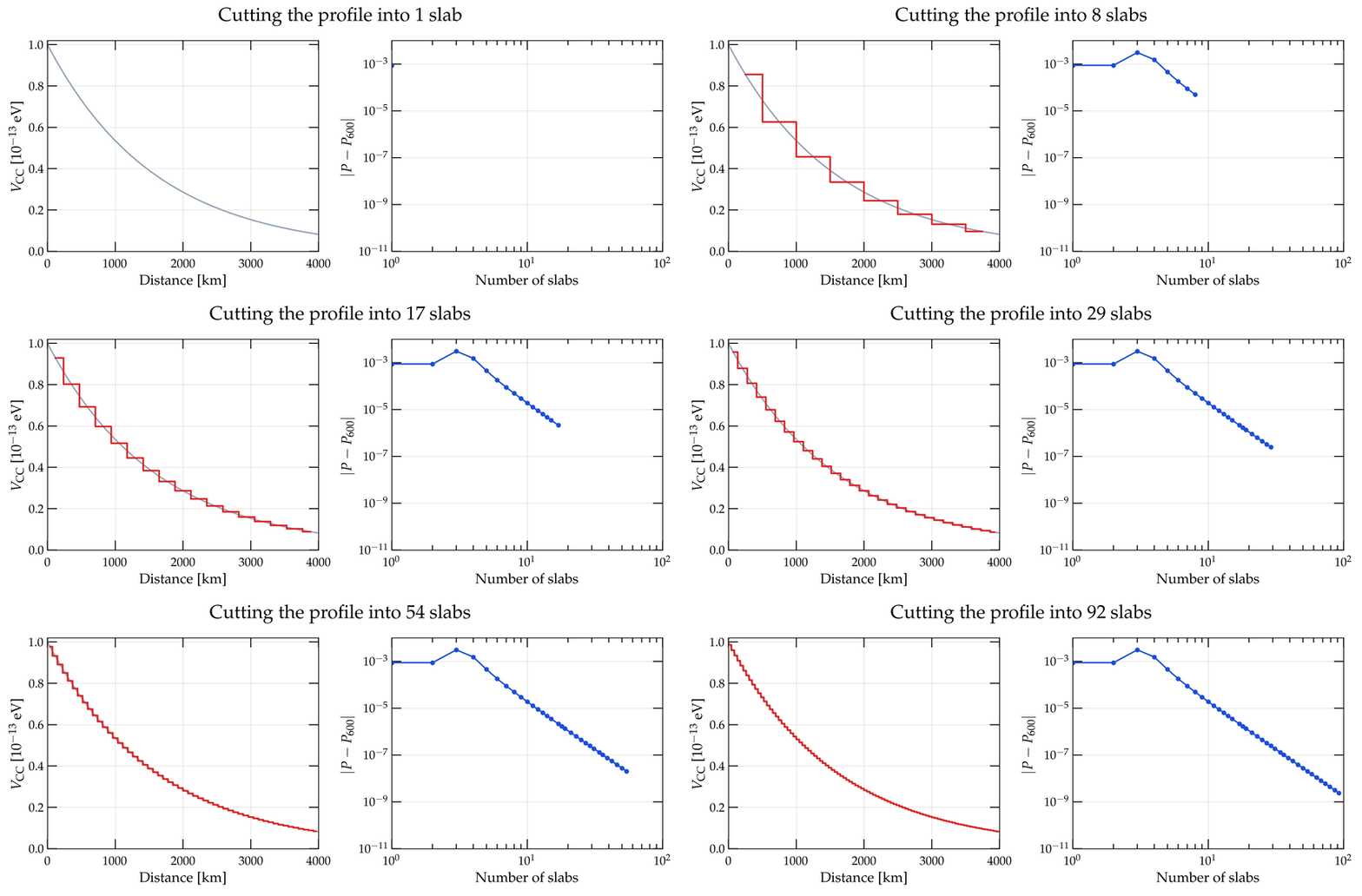
Two measurements make the difference concrete. On a smooth profile, multiplying constant-density slabs together bottoms out near 2.5 × 10⁻¹¹ and then gets worse: past roughly 16 000 slabs, round-off from composing that many matrix products outgrows anything a finer grid buys. Magνs keeps going to 2.9 × 10⁻¹³. And for the Sun, it returns 40 phase-averaged energies in about 0.7 s, where nuSQuIDS needs on the order of ten minutes merely to reach the solver tolerance at which its output is a probability at all.

The two packages deliberately share conventions, units and parameter defaults, so a calculation can be moved from one to the other and used as a cross-check on itself. I do this often.

Some physics it’s meant for

Each of these has a worked notebook in the tutorial gallery, and there is a systematic comparison against other codes in the documentation.

Long-baseline beams and atmospheric neutrinos through the Earth.
Solar neutrinos on a real tabulated model, including the averaged observable.
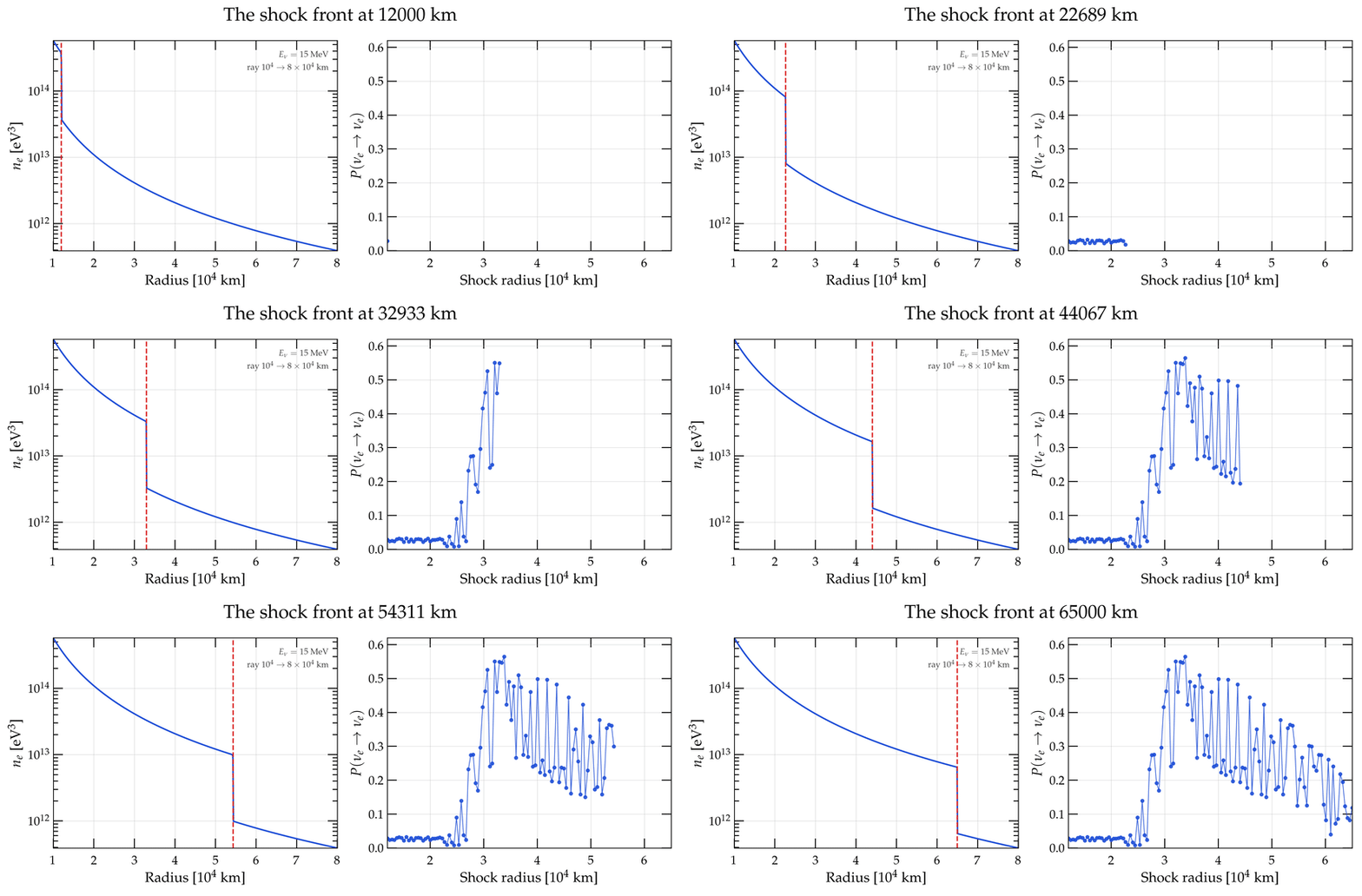
Supernova neutrinos across a shock front — where the width of the front is what decides which method the problem belongs to.
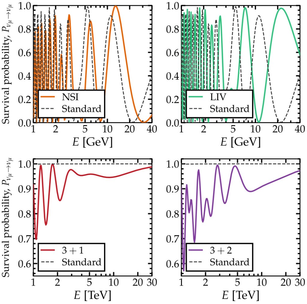
Sterile states (3+1 and 3+2), non-standard interactions, Lorentz-invariance violation.
A Hamiltonian of your own — the escape hatch, and the reason the rest of the list is not exhaustive.

NuOscProbExact 1.11.0: exact neutrino oscillation probabilities for two, three, and now four flavors — on PyPI!

Documentation: https://mbustama.github.io/NuOscProbExact/

Notebooks: https://github.com/mbustama/NuOscProbExact/tree/main/notebooks

Source code: https://github.com/mbustama/NuOscProbExact

PyPI: https://pypi.org/project/nuoscprobexact/

Neutrino oscillation probabilities look like a solved problem until the Hamiltonian stops being the textbook one. There is a closed form in vacuum, and another in two-flavor constant-density matter, and after that it runs out. Add a realistic density profile, a non-standard interaction, a Lorentz-violating operator or a fourth state, and the usual options are to expand in a parameter that may not be small, to diagonalise the Hamiltonian numerically at every point of a grid, or to integrate the Schrödinger equation and hope the step was short enough.

NuOscProbExact does none of these. The Hamiltonian and the time-evolution operator are expanded in the basis of SU(2), SU(3) or SU(4) matrices, and exponentiated analytically using the closure of the algebra. What comes out is a closed form for the probabilities in terms of two or three invariants of the Hamiltonian: no eigenvectors, no numerical diagonalisation, no integration, and no approximation beyond floating-point round-off. Any Hermitian 2×2, 3×3 or 4×4 matrix will do, whatever physics put it there. The method is Ohlsson and Snellman’s, revisited in the 2019 paper; the extension to SU(4) is new since then.

Four flavors is where it stops, for a reason external to neutrino physics: at five, the eigenvalues stop being expressible in radicals — Abel–Ruffini — and the closed form ends with them. Four is exactly what 3+1 needs.

If your reference point is a numerical evolution code, the output is the same object — probabilities, or the evolution operator itself — but with no step size to converge and no dependency beyond numpy. I wrote the first version because adding a model should mean writing down a matrix, not writing a solver. Seven years on it does rather more than it did, and version 1.11.0 now installs with pip.

What it makes easy

Any model, without a new code path. Vacuum, matter, non-standard interactions, Lorentz-invariance violation, sterile states: none of these is a special case in the code. Each is a different matrix handed to the same routine.
A whole scan in one call. A curve against energy or baseline, or a full oscillogram over both, with no Python loop.
Neutrinos through the Earth. Along a zenith angle, or between two of fifteen named sites — CERN–Gran Sasso, Fermilab–Homestake, Tokai–Kamioka and others — with the density profile taken from PREM. Or through any hand-built sequence of slabs of arbitrary width and density, each solved exactly and the operators multiplied.
3+1 sterile scenarios at four flavors, as closed four-state systems rather than as leakage out of the three-flavor block.
The evolution operator itself, not only probabilities, for composing across segments or propagating a density matrix.

Install with:

pip install nuoscprobexact

and, for the optional compiled backend:

pip install "nuoscprobexact[fast]"

MIT licence. Python 3.9 or newer, tested on 3.9 through 3.13, and numpy is the only required dependency: no compiler, nothing to build.

Main features

Accuracy

Cross-checked against independently written code. The probabilities agree with nuSQuIDS to round-off once conventions are matched, and the matter spectrum agrees with the Zaglauer–Schwarzer closed form.
A regression suite of 596 tests, at 100% coverage.

Speed

Arrays instead of loops. Stacks of Hamiltonians, arrays of baselines, or both broadcast together: roughly 20x to 90x faster than the equivalent Python loop, with no extra dependency.
An optional compiled backend. With numba installed, the batched paths run as compiled kernels — answers identical to round-off, used only where it has been measured to win.

What you need to provide

You provide a Hermitian matrix and a baseline, built by hand or with one of the bundled builders for the standard cases. The package returns the exact evolution operator and the probabilities that follow from it, and stops there: no fluxes, no cross sections, no detector response, no fitting. One assumption is worth stating plainly: the Hamiltonian is taken to be time-independent over each segment. A smoothly varying profile can be slabbed, but the step size is then set by the oscillation rather than by the density, and there the documentation points at a Magnus-type method instead.

A minimal example

			
import numpy as np
import oscprob3nu
import hamiltonians3nu
from globaldefs import *
# The vacuum Hamiltonian, without the 1/E factor, so an energy scan
# computes it once
h_vac = hamiltonians3nu.hamiltonian_3nu_vacuum_energy_independent(
    S12_NO_BF, S23_NO_BF, S13_NO_BF, DCP_NO_BF, D21_NO_BF, D31_NO_BF)
# One probability, at 1 GeV over 1300 km
Pee, Pem, Pet, Pme, Pmm, Pmt, Pte, Ptm, Ptt = oscprob3nu.probabilities_3nu(
    np.asarray(h_vac)/1.e9, 1300.0*CONV_KM_TO_INV_EV)
print('Pee = %.5f, Pem = %.5f, Pet = %.5f' % (Pee, Pem, Pet))

		

prints

Pee = 0.92768, Pem = 0.01432, Pet = 0.05800

(The quickstart goes through this more slowly; the recipes page has short, complete snippets for most of what the package can compute, each with real output.)

What is new since 1.0.0

The original announcement, in May 2019, covered the method paper and the code on GitHub. The method has not changed since; almost everything around it has. Whole-array scans arrived in 1.2.0, the optional numba backend in 1.6.0, the Earth and arbitrary layered matter in 1.8.0, and four flavors — oscprob4nu, hamiltonians4nu, the SU(4) expansion — in 1.9.0. In 1.11.0, a non-Hermitian Hamiltonian raises instead of quietly returning probabilities that still sum to one. Along the way, a documentation site and eighteen worked notebooks.

One thing to flag for anyone still running 1.0.0: two fixes in 1.1.0 changed numbers, both at two flavors. probabilities_2nu was missing the h2 contribution to P(νe → νμ), which is invisible whenever the off-diagonal entry is real — so vacuum and constant-density matter were unaffected, but a CP-violating two-flavor Hamiltonian was not — and the two-flavor vacuum Hamiltonian used the opposite sign convention, invisible in vacuum and consequential once a matter potential is added. Three-flavor results from 1.0.0 are unaffected; the changelog has the details.

Some physics it’s meant for

Long-baseline accelerator experiments. DUNE-like baselines through the crust, with matter effects and the CP phase, and the bi-probability ellipses above, which show how matter pushes neutrinos and antineutrinos off the CP-symmetric diagonal. Notebook 05.

Atmospheric neutrinos through the Earth. Zenith-angle scans with the density taken from PREM rather than from a single average value, which is where the mass ordering and the θ23 octant separate. Notebooks 07 and 12.

Sterile neutrinos, 3+1. Short-baseline appearance and disappearance, and the sterile matter resonance through the Earth, with the four states treated as a closed, unitary system rather than as leakage out of the three-flavor block. Notebook 16.

Non-standard interactions and Lorentz-invariance violation. Both enter as extra Hermitian terms added to the vacuum Hamiltonian, so a new operator means a new matrix, not a new solver. Notebook 03.

Unusual matter profiles. Castle-wall and other hand-built profiles, where the arrangement of the matter changes the answer even when the mean density does not — a parametric-resonance effect no constant-density approximation can show. Notebook 08.

Electron stability constrains neutrino time delays

The search for Lorentz-invariance violation (LIV) is one of our best paths toward uncovering the quantum nature of spacetime. One of its most famous potential manifestations is the modification of neutrino propagation speeds.

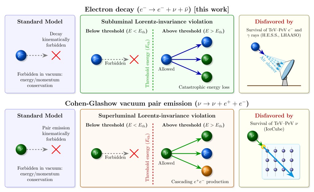
For years, the community has known that superluminal (faster-than-light) neutrinos are heavily constrained. LIV would cause them to rapidly lose energy by radiating electron-positron pairs in a vacuum. Because of this, when anomalous time delays between cosmic neutrinos and gamma rays are observed, phenomenologists have naturally favored subluminal (slower-than-light) LIV propagation as the most viable explanation.

In a new paper co-authored with José Manuel Carmona, José Luis Cortés, Ardit Gkioni, and Maykoll A. Reyes, we demonstrate that this apparent subluminal loophole is actually an illusion.

We show that the same LIV modifications that slow down neutrinos inevitably render high-energy electrons unstable. Under subluminal LIV, electrons undergo a catastrophic decay process: e⁻ → e⁻ + ν + anti-ν. This triggers rapid and severe energy degradation.

By demanding that electrons survive up to the extreme energies we observe in astrophysics—specifically, the 15.5-TeV candidates from H.E.S.S. and the 2.34-PeV electrons inferred by LHAASO in the Crab Nebula—we placed stringent new limits on subluminal LIV.

Our results firmly invalidate the subluminal parameter space previously invoked to explain years-long cosmic neutrino time delays. Consequently, any observable delays must either have purely astrophysical origins, rely on a universal LIV deformation across all particle species, or require physics well beyond the standard effective-field-theory framework.

Read more at:

Electron stability constrains neutrino time delays
Mauricio Bustamante, José Manuel Carmona, José Luis Cortés, Ardit Gkioni, Maykoll A. Reyes
2607.01339 hep-ph

Astrophysical bounds on the high-energy evolution of neutrino mixing

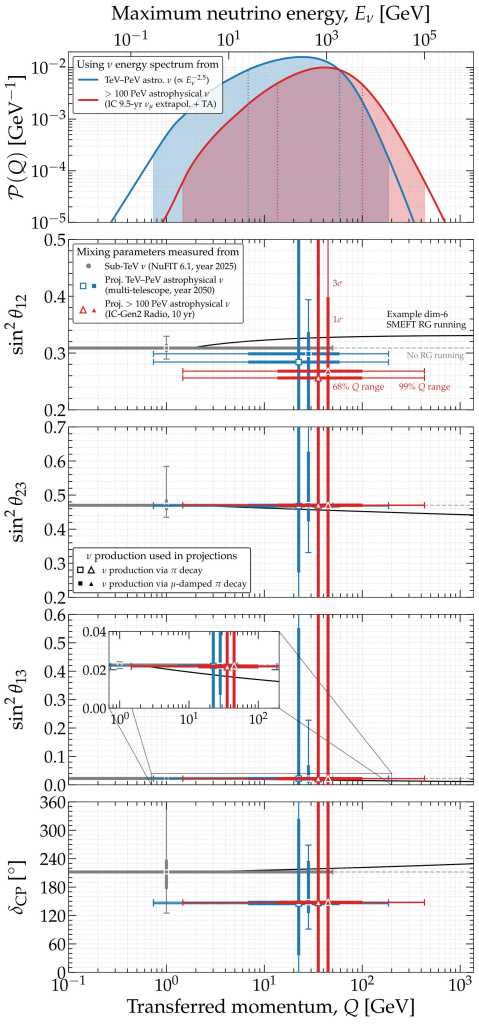
Today, the values of the neutrino mixing angles and mass differences that govern flavor transitions are known to quite high precision. However, we know them exclusively from sub-TeV terrestrial experiments. Because these experiments operate at low transferred momenta (typically, Q ~ few GeV), a fundamental question remains: are the mixing parameters universal constants, or do they evolve at high energies?

Quantum field theory dictates that these parameters should “run” with Q via renormalization group (RG) equations. While this running is negligible in the Standard Model, well-motivated new-physics frameworks, like the Standard Model Effective Field Theory (SMEFT), can accelerate this evolution. Detecting the high-energy running of neutrino mixing parameters would be a smoking-gun signature of new physics.

To access the high-Q regime, we turn to high-energy astrophysical neutrinos, with energies in the TeV–PeV and EeV ranges. They interact in neutrino telescopes via deep inelastic scattering and probe average momentum transfers of Q ~ 20-40 GeV, offering an unprecedented window into this high-Q evolution.

In a new paper with Qinrui Liu and Gabriela Barenboim, we evaluate the power of high-energy astrophysical neutrinos to test the evolution of neutrino mixing. We use the neutrino flavor composition at Earth, i.e., the relative proportions of electron, muon, and tau neutrinos in the diffuse flux. We execute a two-pronged analysis: first, extracting generic high-Q mixing parameters to remain model-agnostic, and second, constraining RG-inducing dimension-6 SMEFT coefficients.

We extract present bounds from the 11.4-year IceCube Medium Energy Starting Events (MESE) sample, published in 2025. Because the uncertainties in current flavor measurements are large, present data cannot yet meaningfully constrain the high-Q mixing parameters or SMEFT operators.

However, the future is promising. For our projections, we simulate the combined detection capabilities of existing (IceCube, Baikal-GVD, KM3NeT) and upcoming (P-ONE, IceCube-Gen2, NEON, TRIDENT, HUNT) optical-Cherenkov neutrino telescopes by the years 2040 and 2050, using both High-Energy Starting Events (HESE) and through-going muons. Crucially, we profile over the unknown astrophysical source flavor composition to ensure our bounds are robust and realistic.

Our results show that by 2040–2050, this global network will achieve the precision necessary to place unprecedented bounds on high-Q mixing (yielding particularly strong constraints in the 23 and 13 sectors). Furthermore, if the astrophysical neutrinos are produced via muon-damped pion decay, these telescopes will be capable of placing limits on individual SMEFT coefficients at a new-physics scale of 1 TeV, easily translatable to other energy scales.

We also forecasted the sensitivity of ultra-high-energy (UHE) radio arrays, such as the planned IceCube-Gen2 radio array. Counterintuitively, we found that despite UHE neutrinos possessing much higher energies, they yield drastically weaker constraints than their TeV–PeV counterparts. This is driven both by the logarithmic scaling of the RG evolution and by the vast experimental uncertainties inherent to radio-based flavor tagging.

Read more at:

Astrophysical bounds on the high-energy evolution of neutrino mixing
Mauricio Bustamante, Qinrui Liu, Gabriela Barenboim
2604.14409 hep-ph

Measuring neutrino mixing above 1 TeV with astrophysical neutrinos

Today, the values of the neutrino mixing angles that govern flavor transitions are known to percent precision (the Dirac CP-violation phase is known much more poorly). However, these values are inferred exclusively from sub-TeV neutrino experiments. No measurement of the mixing parameters exists at the TeV scale and above. There, new-physics effects whose intensity grows with neutrino energy could modify the effective neutrino mixing. High-energy astrophysical neutrinos, with TeV-PeV energies, are primed for such measurements.

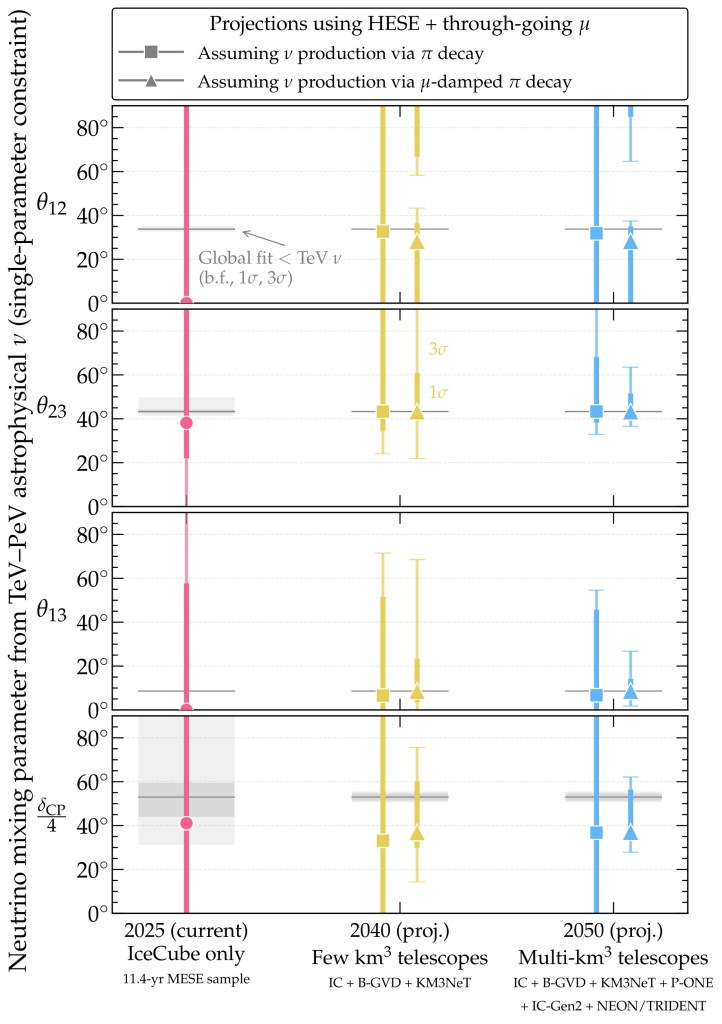
In a new paper with Qinrui Liu and Gabriela Barenboim, we have assessed in detail the power in these neutrinos to test mixing above 1 TeV, today and in the future. Concretely, we have extracted values of the four neutrino mixing angles (𝛉₁₂, 𝛉₂₃, 𝛉₁₃) and the CP-violation phase (δ_CP) from the flavor composition of high-energy astrophysical neutrinos, i.e., the proportion of electron, muon, and tau neutrinos in their diffuse flux.

We extract present bounds on the mixing parameters from the 11.4-year IceCube Medium Energy Starting Events (MESE) sample, published in 2025. We find that the uncertainty in the measurement is too large to claim meaningful sensitivity to the mixing parameter.

For our projections, we use multi-neutrino-telescope combinations using projected detection rates at existing (IceCube, Baikal-GVD, KM3NeT) and future (P-ONE, IceCube-Gen2, NEON, TRIDENT, HUNT) neutrino telescopes. For these, we combine High Energy Starting Events (HESE) and through-going muons. Our projections show clear sensitivity to 𝛉₂₃ and 𝛉₁₃ (and, if neutrino production occurs via muon-damped pion decay, to δ_CP). This establishes benchmarks for the minimum size that new-physics modifications to the mixing parameters must have in order to be detectable.

Read more at:

Measuring neutrino mixing above 1 TeV with astrophysical neutrinos
Mauricio Bustamante, Qinrui Liu, Gabriela Barenboim
2602.14308 hep-ph

No Flavor Anisotropy in the High-Energy Neutrino Sky Upholds Lorentz Invariance

Do neutrinos of different flavors have different preferred directions? If so, this would mean that Lorentz invariance is violated, something that is posited by some theories of quantum gravity. In them, Lorentz-invariance violation (LIV) would become more prominent the higher the energies involved.

Motivated by this, we look for signs of this flavor-dependent LIV using the high-energy astrophysical neutrinos seen by IceCube, with energies in the TeV-PeV range.

If LIV exists, the neutrinos would be affected by their interaction with a pervasive LIV field that couples differently to different neutrino flavors. As a result, the sky distributions of high-energy astrophysical electron, muon, and tau neutrinos arriving at Earth would be anisotropic.

In a new paper led by PhD student Bernanda Telalovic, we look for these high-energy neutrino flavor anisotropies in IceCube data, specifically, in the public 7.5-year sample of High-Energy Starting Events (HESE). We do this using the methods introduced in an earlier paper of ours (2310.15224).

We find no evidence for the patterns of flavor anisotropy expected from LIV, and so we place new upper limits on hundreds of parameters regulating Lorentz-invariance violation within the Standard Model Extension. We explore LIV operator dimensions from 2 to 8, each with a different dependence on neutrino energy and introducing different forms of flavor anisotropy.

For many of them, we improve upon existing limits—on account of using higher energies—or place limits for the first time ever:

Our new upper limits on the LIV parameters are available in digital form for download at 68%, 95%, and 99% C.L. GitHub, here.

Read more at:

No Flavor Anisotropy in the High-Energy Neutrino Sky Upholds Lorentz Invariance
Bernanda Telalovic, Mauricio Bustamante
2503.15468 astro-ph

Global monitoring for high-energy neutrino astronomy

Genuine high-energy neutrino astronomy needs many and varied astrophysical sources. But finding sources is hard, especially having only one km-scale neutrino telescope in operation. This is changing fast, though, thanks to the ongoing construction of KM3NeT and Baikal-GVD, but transformative progress will require us to think globally.

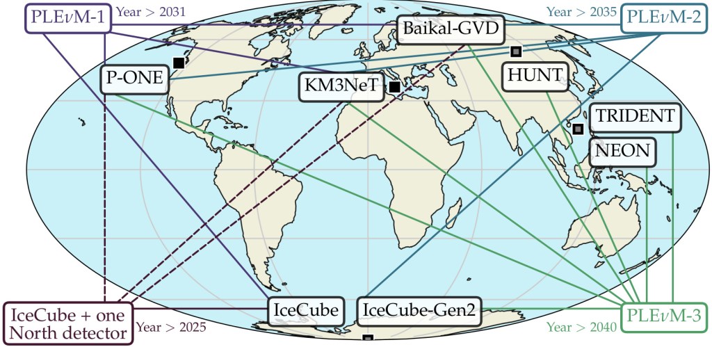
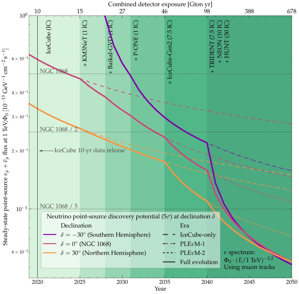
In a new paper, led by Lisa Schumacher, we show that, in the next 10-20 years, IceCube + Baikal-GVD, KM3NeT, IceCube-Gen2, P-ONE, TRIDENT, NEON, & HUNT, taken together in PLEnuM, could allow us to make global high-energy neutrino monitoring a reality. Together, they will increase the global rate of neutrino detection by up to 30 times and continuously monitor the entire sky.

To showcase this, we focus on one of the most prominent science cases in high-energy neutrino astronomy: finding steady-state sources. A combined analysis of global data will expedite source discovery—in some cases, by decades—and enable the detection of fainter sources anywhere in the sky, discovering up to tens of new neutrino sources.

This is seen, for example, in our forecasts for the evolution of the discovery potential of neutrino sources that have a soft spectrum (like NGC 1068), placed in different locations in the sky:

The PLEnuM tools used to obtain the results in our paper (plus more) are open-source and available on GitHub, here.

Read more at:

Beyond first light: global monitoring for high-energy neutrino astronomy
Lisa Johanna Schumacher, Mauricio Bustamante, Matteo Agostini, Foteini Oikonomou, Elisa Resconi
2503.07549 astro-ph

IV NBI Neutrino Summer School “Here, There & Everywhere”

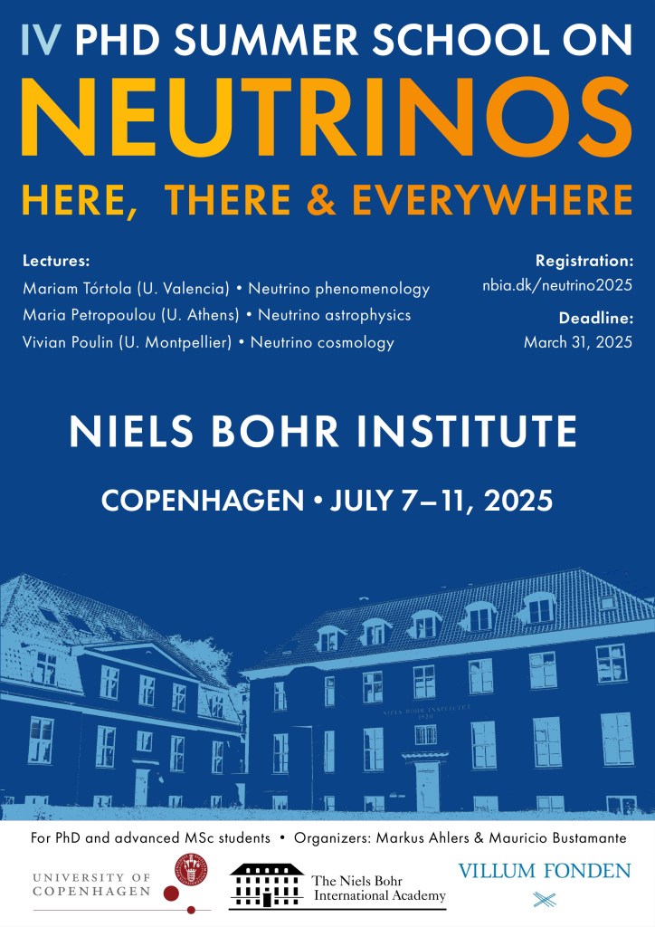
Registration is now open for the fourth edition of our NBI Neutrino Summer School, “Here, There & Everywhere”.

Like in previous editions (2021, 2022, 2023), the school is aimed at PhD students and advanced MSc students from all over the world that work on neutrinos, are planning to work on them, or are simply interested in them! The school is a one-week series of lectures on neutrino phenomenology, astrophysics, and cosmology delivered by carefully chosen world experts on these subjects.

When? July 7-11, 2025

Where? Niels Bohr Institute, Copenhagen, Denmark

How to register? Go to our Indico page here

Registration deadline: March 31, 2025 (register early!)

Can you present a student talk? Accepted in-person participants are encouraged to submit an abstract

Is there a participation fee? Yes, there is a fee of 130 EUR for in-person participants

Questions? Find our contact information (Markus Ahlers, Mauricio Bustamante) on the Indico page

The school provides lunch (Monday to Friday), two coffee breaks a days, reception and a school dinner.

MITP Summer School 2024 Multi-Messenger Lecture Videos

The video recordings of my four-lecture mostly blackboard course on multi-messenger astrophysics at the 2024 MITP (Mainz Institute for Theoretical Physics) Summer School “Crosslinks of Early Universe Cosmology” are now on YouTube.

Part 1:

Part 2:

Part 3:

Part 4: