What twelve years of daily arXiv picks say about my reading

Standard

How has what I read changed over twelve years?

Since February 2014, I have kept a daily list of the arXiv preprints that I find interesting. Since October 2017, the list has been public on this site as My daily arXiv picks. I recently gathered all of it, 18,169 papers, into one table and looked at what it says. Here are the highlights.

I pick three times as many papers. In 2014 I picked 704 papers. In 2025 I picked 2,166, and 2026 is at 1,910 so far. I have also become much stingier with two stars, which I use for papers that are very relevant to my own work: they made up a quarter of my picks in 2014–2017, and about 2% since 2019.
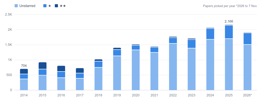
Stacked bar chart of the number of arXiv papers picked per year from 2014 to 2026, split into unstarred, one-star and two-star picks.
Papers I picked each year, split by star level. One star marks a paper I found especially interesting; two stars, one that is very relevant to my own work. 2026 runs to November 7.

From astro-ph towards hep-ph. In 2014, 62% of my picks were listed in astro-ph and 16% in hep-ph. In 2026, the split is 44% and 39%. Most of the shift happened between 2017 and 2021.
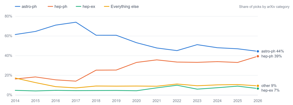
Line chart of the share of picks in astro-ph, hep-ph, hep-ex and other arXiv categories from 2014 to 2026.
Share of my picks in each arXiv category, by year.

What I read and what I star have drifted apart. To compare topics fairly across years, I compared how often I star papers on a topic with how often I star papers overall in the same years. The topics I star most often are all about high-energy neutrinos: the 220-PeV KM3NeT event KM3-230213A (3.3 times my average star rate), the Glashow resonance (3.0), NGC 1068 and Seyfert galaxies (2.8), and high-energy astrophysical neutrinos in general (2.3).

Dark matter, on the other hand, is the single largest topic I pick: 3,094 papers, about a fifth of my picks in recent years. Yet I star it at only 0.8 times my average rate. Axions grew from under 1% of my picks to about 5%, and machine learning from almost nothing to 4% in 2026, but I rarely star either. Gamma-ray bursts went the other way, from about 11% of my picks in 2014–2017 to 2% in 2025–2026.
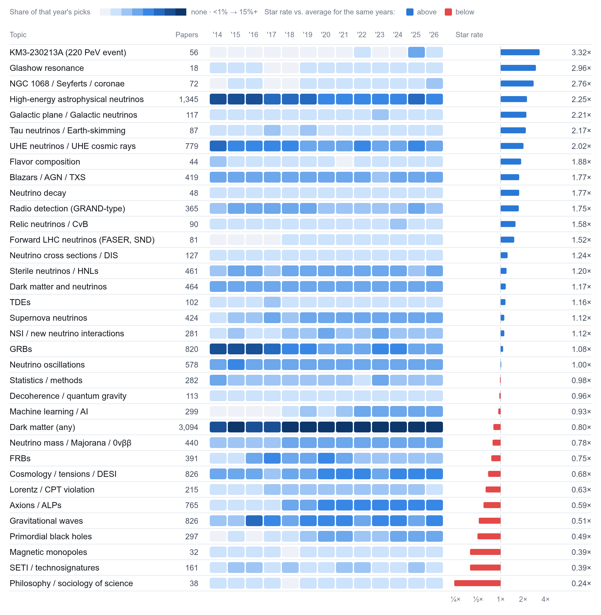
Table of 34 topics showing each topic’s share of picks per year as colored cells, and how often papers on each topic are starred relative to the average.
Each row is a topic, assigned by keywords in paper titles. The colored cells show the share of each year’s picks on that topic. The bars show how often I star papers on that topic compared with my average for the same years. Click to enlarge.

Explore the list. I put all 18,169 picks in a searchable page. You can search by title, author, or arXiv identifier, and filter by stars, year, arXiv category, or topic.

A few caveats: topics are assigned by keyword matches on paper titles, so they are approximate, and years come from arXiv identifiers.

I put together the analysis and the searchable page with the help of Claude.

PyFC: a Python framework for Feldman-Cousins confidence intervals

Standard

Links

Setting a confidence interval sounds like a solved problem, until you actually have to do it. Deciding whether to quote a two-sided interval or a one-sided upper limit after looking at the data — the classic “flip-flopping” — breaks coverage, and near a physical boundary (a mass, a cross section, a flavor fraction) the usual construction can return an empty or unphysical interval. Feldman and Cousins’ 1998 unified approach fixed this by using the likelihood-ratio ordering principle to let the data decide the interval’s shape automatically, with guaranteed coverage throughout. It has become the standard approach for small-signal counting experiments across particle and astroparticle physics — but implementing it correctly, especially in more than one dimension and with realistic, finite-statistics systematics, is a substantial piece of software to get right.

That’s what I built PyFC to handle — it supports binned and unbinned likelihoods natively, in the same framework, rather than treating one as a special case of the other. Given a likelihood, it runs the Monte Carlo pseudo-experiments needed to empirically calibrate the profile-likelihood-ratio distribution, and returns exact-coverage Feldman-Cousins intervals and contours — in one or several dimensions, on a laptop or on a cluster. I kept needing exactly this — correct-coverage contours for neutrino mixing-parameter extractions and HNL coupling limits in my own papers — and rewriting the toy-generation machinery from scratch for each project wasn’t sustainable.

If your reference point is ROOT/RooStats’ FeldmanCousins calculator: PyFC does the same statistical job with no ROOT dependency — plain NumPy/SciPy arrays and a pip install, so it drops straight into a normal Python analysis.

Main features

PyFC is built for speed, flexibility, and accuracy — none traded off for the others.

Speed

  • Parallel processing by default. Binned fits use Numba/NumPy C-extensions with GIL-bypassing thread pooling; unbinned fits parallelize across CPU cores via Python’s multiprocessing (ProcessPoolExecutor). Toy generation — normally the bottleneck in any Feldman-Cousins analysis — scales with however many cores you give it.
  • No wasted compute. Adaptive early-stopping (adaptive_toys) and batched dispatch (toy_batch_size) stop generating toys once the result is statistically clear, instead of running a fixed, oversized number every time.
  • Resumable. Checkpointing saves state after each parameter/pair scan, so a run killed by a cluster walltime limit picks up where it left off instead of restarting from zero.

Flexibility

  • Native binned and unbinned support, in one framework. Poisson binned data — including arbitrary N-dimensional, even non-contiguous, histograms — and Extended Unbinned Maximum Likelihood models are both first-class, not one bolted onto the other.
  • A choice of optimizer. Gradient-based SciPy (L-BFGS-B), nested sampling via UltraNest, brute-force grid scans, or a Hybrid strategy that uses UltraNest’s robustness for the one global fit and SciPy’s speed for the many conditional fits that follow.
  • Physical constraints between parameters, not just per-parameter boxes. bounds_func and constraints express joint or simplex conditions (e.g. a + b ≤ 1) that an independent [lo, hi] range per parameter can’t capture.

Accuracy

  • Coverage that’s actually exact. The test-statistic distribution is derived empirically from generated toys rather than assumed from Wilks’ theorem, and disconnected accepted regions are reported as separate intervals instead of being silently merged into one.
  • Finite-Monte-Carlo corrections for limited simulation statistics, so a small MC background template doesn’t bias the result.

Also: optional 2D grid sparsification for faster contours, and an interactive CLI for generating run configurations.

Open source (GPLv3), Python 3.8+.

What you need to provide

You bring the physics, PyFC handles the statistics:

  • A physics mapper — for binned data, a compute_rates_func that maps your free parameters to expected bin counts and variances; for unbinned data, that plus pdf_components (one function per signal/background component) and a generate_toy_func for parametric bootstrapping.
  • Your data — a histogram (any shape, any dimension) or an array of events.
  • grids — the scan grid for each free parameter, plus bounds_func/constraints for any joint constraints between them.
  • A config — confidence level, toy settings, checkpointing, and the optimizer strategy (grid, scipy, ultranest, or hybrid), built interactively with the CLI or as a JSON file.

Call compute_fc_intervals and PyFC takes care of the rest: toy generation, parallelization, checkpointing, and exact-coverage intervals out the other end — no hand-rolled Monte Carlo loop required.

A minimal example

For a binned Poisson analysis with a signal and a background component:

import numpy as np
from numba import njit
from pyfc import compute_fc_intervals
# A fixed expected-shape array, captured via closure (not itself a fit parameter)
expected_shape = np.array([0.1, 0.5, 2.0, 5.0])
@njit(fastmath=True, nogil=True)
def compute_rates(params):
"""Map parameters -> expected bin counts (mu) and variances (sigma2)."""
mu = params[0] * params[1] * expected_shape + params[2] # signal (rate x efficiency) + background
sigma2 = mu # Poisson variance
return mu, sigma2
observed_counts = np.array([20, 7, 2, 0]) # data — any shape, not just 1D
grids = [
np.linspace(1e-9, 1e-7, 20), # param_1
np.linspace(2.0, 3.0, 15), # param_2
np.linspace(0.8, 1.2, 10), # param_3
]
# results: exact-coverage FC intervals/contours for param_1-3, plus the
# underlying profile-likelihood scan and toy statistics behind them
results = compute_fc_intervals(
data=observed_counts,
grids=grids,
compute_rates_func=compute_rates,
**config, # confidence level, toy settings, strategy — see Configuration
)

(See the Quick Start Guide for the full binned and unbinned walkthroughs, with real output.)

Install with:

pip install PyFeldmanCousins

Some physics it’s meant for

Feldman-Cousins intervals matter most exactly where physics tends to live: near a boundary, with a marginal signal, where Gaussian/Wilks assumptions don’t hold. A few non-trivial cases PyFC is a natural fit for:

  • Astrophysical neutrino flavor composition. The flavor fractions (f_e, f_μ, f_τ) of the diffuse high-energy neutrino flux live on a simplex, f_e + f_μ + f_τ = 1 — precisely the joint-constraint case that bounds_func/constraints were built for. Feldman-Cousins contours on the flavor triangle are the standard way to compare an IceCube-like measurement against competing production scenarios (pion decay, muon-damped decay, neutron decay) and BSM flavor physics. Worked through hands-on in tutorial notebook 06.
  • Heavy Neutral Lepton searches at beam-dump experiments. A null result from a fixed-target experiment like SHiP constrains the active-sterile mixing |U|² as a function of HNL mass — an upper limit sitting right against the |U|² ≥ 0 boundary, often with disconnected sensitivity islands where the excluded region reappears at higher mass — see tutorial notebook 04 for how PyFC reports these correctly.
  • Dark matter direct-detection cross-section limits. The textbook case: a handful of candidate events over an uncertain background, where the interval needs to turn two-sided smoothly if a real excess ever shows up, instead of flip-flopping into an artificially tight one. The quickstart tutorial notebook works through essentially this case end to end.
  • Accelerator and reactor neutrino oscillations. Joint 2D regions on (Δm², sin²2θ) — this is literally the original 1998 Feldman-Cousins worked example, and still a good stress test for comparing the grid, SciPy, and Hybrid strategies — see tutorial notebook 05.
  • Neutrinoless double-beta decay. Binned searches for a peak near the Q-value, where the finite-MC correction matters because the simulated background templates are themselves statistics-limited — see tutorial notebook 04 for the correction on vs. off.